1 Introduction
How large can the pathwidth of a sparse graph be? For graphs of maximum degree \(3\) the best upper bound has stood for twenty years: Fomin and Høie (Fomin and Høie 2006) proved that they have pathwidth at most \(\frac16n+o(n)\), where \(n\) is the number of vertices. We prove that graphs of maximum degree \(3\) have pathwidth at most \[c_{3}\, n+o(n),\qquad c_{3}=\frac{3}{4\pi}\arccos\frac56\approx 0.13982,\] with corresponding improvements at every degree, per edge, and in the running times of the exact algorithms built on these bounds.
The proof of the old bound cuts the graph into two halves along a bisection with about \(\frac n6\) edges, which exists by the theorem of Monien and Preis (Monien and Preis 2006 Theorem 1), and then decomposes each half with a prescribed boundary. Each of the two steps needs width about \(\frac n6\). The per-degree bounds of Fomin, Gaspers, Saurabh and Stepanov (Fomin et al. 2009) and of Edwards and McDermid (Edwards and McDermid 2015) extend the bound to all graphs by deleting vertices of large degree, and the per-edge bound \(\frac{13}{75}m\) of Scott and Sorkin (Scott and Sorkin 2007), as well as the bound \(\frac m{5.769}\) of Kneis, Mölle, Richter and Rossmanith (Kneis et al. 2009), also follows from these per-degree bounds. Many exact algorithms for sparse instances run a dynamic program over a decomposition of such a width, and their running times are stated through these constants. We replace bisection by a different construction: a threshold sweep through a correlated Gaussian labeling of the vertices. Counting only the edges that cross a threshold of this sweep already gives pathwidth at most \(\left(\frac{3}{2\pi}\arcsin\frac13\right)n+o(n)\approx0.1623n\), below \(\frac n6\), with a short complete proof whose probabilistic tools are the random-hyperplane lemma of Goemans and Williamson (Goemans and Williamson 1995) and Chebyshev’s inequality (Theorem 3.1).
1.1 Width bounds
Throughout, graphs are finite and simple, \(n=|V(G)|\), \(m=|E(G)|\), \(n_d=n_d(G)\) is the number of vertices of degree \(d\), and \(\Delta(G)\) is the maximum degree. Every remainder \(o(n)\) (or \(o(m)\)) stands for a function of \(n\) (or \(m\)) alone, the same for all graphs in the stated class. Since every path decomposition is a tree decomposition, all bounds also hold for treewidth.
Theorem 1.1 (bounded degree). Let \(G\) be a graph with \(n\) vertices.
(a) If \(\Delta(G)\le3\), then \(\mathop{\mathrm{pw}}(G)\le c_{3}\,n+o(n)\), where \(c_{3}=\frac{3}{4\pi}\arccos\frac56\approx0.13982\).
(b) If \(\Delta(G)\le4\), then \(\mathop{\mathrm{pw}}(G)\le F_4\,n+o(n)\), where \(F_4\approx0.24577\) is the maximum over the threshold of an explicit Gaussian integral, the ideal \(4\)-star function (2.2).
Lean proof, (a) without hypotheses and (b) under H1: C3.c3MainClaim, T2.target2a (what is formalised)
Part (a) is Theorem 8.1, proved in Section 8, and part (b) is Theorem 7.1(a), proved in Section 7. The constant \(c_{3}\) also bounds two other width parameters. The bisection width \(\operatorname{bw}(G)\) is the minimum number of edges between the two sides of a partition of \(V(G)\) into parts whose sizes differ by at most one, and the cutwidth \(\operatorname{cw}(G)\) is the minimum, over all linear orderings of \(V(G)\), of the maximum number of edges joining a vertex before a gap of the ordering to a vertex after it.
Corollary 1.2 (bisection width and cutwidth). Every graph \(G\) with \(\Delta(G)\le3\) satisfies \(\operatorname{bw}(G)\le\operatorname{cw}(G)\le c_{3}\,n+o(n)\).
The corollary follows from Theorem 1.1(a) through the chain \(\operatorname{bw}(G)\le\operatorname{cw}(G)\le\mathop{\mathrm{pw}}(G)+2\) for maximum degree \(3\): bisection width is at most cutwidth (Dı́az, Petit, and Serna 2002 Lemma 2.4), cutwidth equals the search number for maximum degree \(3\) (Makedon and Sudborough 1989 Corollary 3.3), the search number is at most the vertex separation number plus \(2\) (Ellis, Sudborough, and Turner 1994 Theorem 2.1) (see also (Bodlaender 1998)), and vertex separation equals pathwidth (Kinnersley 1992 Theorem 3.1).
For bisection width, Corollary 1.2 improves the bound \(\frac n6+o(n)\) that Monien and Preis (Monien and Preis 2006 Theorem 1) proved for cubic graphs. For cutwidth, the previous bound \(\frac n6+o(n)\) followed from the theorem of Fomin and Høie by the same relations. Corollary 10.2 computes, in deterministic time \(n^{2+o(1)}\), an ordering of cutwidth at most \(c_{3}n+o(n)\) and a bisection with at most that many edges between its sides.
The constant \(c_{3}\) is not new as a bisection constant: Lichev and Mitsche (Lichev and Mitsche 2023) proved that random cubic graphs have bisection width at most \(c_{3}n+o(n)\) asymptotically almost surely (stated there as \(0.139822n\)), and at least \(0.103295n\). What is new is that the same constant holds for every graph of maximum degree \(3\), and for pathwidth. The lower bound for random cubic graphs gives pathwidth at least \(0.103295n-2\). We conjecture (Conjecture 15.1) the upper bound \(\mathop{\mathrm{pw}}(G)\le(c_{3}-3p_{\mathrm{ch}})n+o(n)\approx0.1322n+o(n)\) for cubic graphs.
The simplest form of our method, which counts the edges that cross a threshold, also bounds the cutwidth for larger maximum degree. Theorem 3.6 in Section 3 shows that every graph \(G\) with \(\Delta(G)\le p\) has cutwidth at most \(\gamma_pm+o(n)\), where \(\gamma_p=\frac1\pi\arccos\frac{2\sqrt{p-1}}p\). For \(\Delta(G)\le4\) this is \(\frac m6+o(n)\le\frac n3+o(n)\), which improves the second bound of Monien and Preis (Monien and Preis 2006 Theorem 2), \(\frac{2n}5+o(n)\) for the bisection width of \(4\)-regular graphs; for \(\Delta(G)\le5\) it is at most \(0.5121n+o(n)\). For \(p\in\{4,5\}\) the orderings can be computed in deterministic polynomial time (Theorem 10.3). The bound also gives the edge isoperimetric number (Section 3.6).
For graphs with vertices of all degrees we prove one bound per vertex, with a closed-form coefficient for every degree, and one bound per edge.
Theorem 1.3 (all graphs). Every graph \(G\) satisfies \(\mathop{\mathrm{pw}}(G)\le\sum_{d\ge 3}a_d\,n_d+o(n)\) for the sequence \[a_d= \begin{cases} \dfrac{3d-4}{32} & \text{for } 3\le d\le 6,\\[8pt] 1-\dfrac{111}{28\,(d+1)} & \text{for } 7\le d\le 10,\\[8pt] 1-\dfrac{4}{d+1} & \text{for } d\ge 11. \end{cases}\]
Lean proof under H3: T4.target4 (what is formalised)
The first coefficients are \((a_3,a_4,a_5,a_6)=\bigl(\tfrac{5}{32},\,\tfrac14,\,\tfrac{11}{32},\,\tfrac{7}{16}\bigr)\); rounded up to four decimals, \((a_3,\dots,a_{11})\) is \((0.1563,\,0.2500,\,0.3438,\,0.4375,\,0.5045,\,0.5596,\,0.6036,\,0.6397,\,0.6667)\).
Corollary 1.4 (edges). Every graph \(G\) satisfies \(\mathop{\mathrm{pw}}(G)\le \frac{7}{48}\, m+o(n)\).
Lean proof under H3: T4.target5 (what is formalised)
Both are proved in Section 9. Table 1 compares the coefficients with the previous ones. The relative improvement is largest at degree \(4\): from \(\frac13\) to \(\frac14\) per vertex of degree \(4\), and to \(F_4\approx0.2458\) for the whole class \(\Delta\le4\). The per-edge bound comes from the degree \(d\) that maximizes \(\frac{2a_d}{d}\). For the previous coefficients this is \(d=5\), with \(\frac{13}{75}\approx0.1733\); for ours it is \(d=6\), with \(\frac{2a_6}{6}=\frac{7}{48}\approx0.1458\). For large degrees the coefficients of Theorem 1.3 approach \(1\) as \(1-\frac{4}{d+1}\), against \(1-\frac{3.5}{d+1}+O(d^{-3})\) for the coefficients \(g_{1/6}(d)\) of Edwards and McDermid (Edwards and McDermid 2015).
Table 1: Upper bounds on pathwidth, without the lower-order terms: per vertex for the classes \(\Delta\le3\) and \(\Delta\le4\) (Theorem 1.1), per vertex of degree \(d\) (Theorem 1.3) and per edge (Corollary 1.4). Previous bounds: (Fomin and Høie 2006) for \(\Delta\le3\); (Fomin et al. 2009) for \(\Delta\le4\) and for degrees \(3\) to \(6\); the coefficients \(g_{1/6}(d)\) of (Edwards and McDermid 2015) for \(d\ge7\); and \(\frac{13}{75}m\) from (Scott and Sorkin 2007) ((Kneis et al. 2009) state \(\frac m{5.769}\)). Decimals are rounded to four places. In Theorem 1.3 the coefficient of degree \(3\) exceeds \(c_{3}\): the triple behind it trades a larger coefficient at degree \(3\) for smaller ones at degrees \(4\) and \(5\), and for \(\Delta\le3\) Theorem 1.1(a) applies.
| \(\Delta\le3\) | \(\Delta\le4\) | \(d=3\) | \(d=4\) | \(d=5\) | \(d=6\) | \(d=7\) | \(d\ge11\) | per edge | |
|---|---|---|---|---|---|---|---|---|---|
| previous | \(\frac16\) | \(\frac13\) | \(\frac16\) | \(\frac13\) | \(\frac{13}{30}\) | \(\frac{23}{45}\) | \(0.5698\) | \(1-\frac{3.5}{d+1}+O(d^{-3})\) | \(\frac{13}{75}\) |
| this paper | \(0.1398\) | \(0.2458\) | \(\frac{5}{32}\) | \(\frac14\) | \(\frac{11}{32}\) | \(\frac{7}{16}\) | \(0.5045\) | \(1-\frac{4}{d+1}\) | \(\frac{7}{48}\) |
Theorem 1.3 is one of several bounds of this form. Section 9 states all coefficient vectors of the paper as pathwidth sequences, among them the pair \((c_{3},0.2627)\) for maximum degree \(4\) (Theorem 8.2), and extends each of them to all degrees by a bootstrap lemma. It also shows that the bootstrap of \((\frac5{32},\frac14,\frac{11}{32})\), which Theorem 1.3 rounds up to closed forms, has the smallest coefficient at every degree \(d\ge5\).
The method in one paragraph.
We give every vertex a Gaussian label, a weighted sum of independent standard normal variables over a ball around the vertex with critically decaying weights, and sweep a threshold through the labels. The vertex separation layout turns the sweep into a path decomposition whose width is the size of the largest frontier, the set of vertices on one side of the threshold with a neighbor on the other side. Whether a vertex lies in a frontier depends only on the labels of its closed neighborhood, a star. We bound that probability from above by the one for an explicit ideal star, using that the regular simplex minimizes Gaussian orthant probabilities. A threshold has two frontiers: its outer frontier is the set of vertices above the threshold with a neighbor at or below it, and its inner frontier is the set of vertices at or below the threshold with a neighbor above it. For maximum degree \(3\), outer frontiers at every threshold give width about \(0.1402n\); inner frontiers for thresholds below the median and outer frontiers above it lower the width to \(c_{3}n+o(n)\). Figure 1 shows the two frontier curves of the ideal star and the envelope that bounds the median-switched sweep; Section 2 develops these ideas.
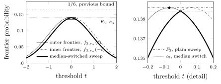
Figure 1: The ideal \(3\)-star function \(f_{3,r_*}\) at the cubic correlation \(r_*=\frac{2\sqrt2}3\), computed from the ideal star function (2.2) of Section 2, and its reflection. The right panel enlarges the box drawn in the left panel, and the dotted line at \(1/6\) is the previous bound for maximum degree \(3\) (Fomin and Høie 2006). The plain sweep has width at most \(F_3n+o(n)\approx0.1402n\), where \(F_3\) is the maximum of the thin solid curve, attained at \(t\approx-0.068\) (filled dot). The median-switched sweep keeps inner frontiers for \(t<0\) and outer frontiers for \(t>0\). It has width at most \(c_{3}n+o(n)\approx0.1398n\), where \(c_{3}\) is the maximum of the thick envelope, attained at \(t=0\) (open dot): by the switch lemma (Section 2.4), the passage from inner to outer frontiers at \(t=0\) adds nothing at leading order.
1.2 Algorithms and consequences
The proofs of the width bounds are probabilistic. Section 10 makes them algorithmic: it approximates the Gaussian variables by a finite rational probability distribution and derandomizes by the method of conditional expectations. Theorem 10.1 there is the precise form of the following theorem and states the computational model.
Theorem 1.5 (computing the decompositions). Let \(\beta(G)\) be any of the bounds of Theorems 1.1 and 1.3, Corollary 1.4, Theorems 7.1, 7.2, 8.2 and 9.2 and Corollary 9.5 (for Theorem 7.1(a), \(F_4n\)), without its remainder term. For every graph \(G\) in the class of the bound, a path decomposition of \(G\) of width at most \(\beta(G)+o(n)\) can be computed in deterministic time \(n^{2+o(1)}+O(n(n+m))\), and by a Las Vegas algorithm in expected time \(n^{1+o(1)}+O(n(n+m))\).
Part II follows the new constants through the literature of exact algorithms. The five most striking consequences are the following, and Table 2 lists forty-five rows of bounds that, as far as we know, two recent preprints would not supersede (see the paragraph on the Exponential Time Hypothesis below). To our knowledge, each bound of Theorem 1.6 and Table 2 is the fastest known for its problem and graph class (for a deterministic bound, among deterministic algorithms), subject to the table notes.
Theorem 1.6 (faster exact algorithms). Polynomial factors are omitted; \(r\) is the domain size, \(n\) the number of variables or vertices, \(m\) the number of constraints or edges and \(k\) the pattern size. The following problems can be solved in the stated time.
(i) Minimum Weight Dominating Set and #Minimum Weight Dominating Set, for vertex weights with polynomially many distinct subset sums, in time \(O(1.4815^n)\).
(ii) Max \((r,2)\)-CSP in time \(r^{7m/48+o(m)}\).
(iii) The number of subgraphs of a graph that are isomorphic to a given pattern with \(k\) edges, in time \(k^{O(k)}n^{7k/48+o(k)}\).
(iv) Permutation Pattern Matching, in time \(2^{O(k)}n^{253k/1215+o(k)}\), and \(k\)-opt Optimization for the traveling salesperson problem, in time \(O(n^{(253/1215+\varepsilon_k)k})\) with \(\varepsilon_k\to0\) as \(k\to\infty\).
(v) On graphs of maximum degree \(4\), Feedback Vertex Set by a Monte Carlo algorithm in time \(O(1.2600^n)\) and deterministically in time \(O(1.4853^n)\), and the traveling salesperson problem deterministically in time \(O(1.4214^n)\); on graphs of maximum degree \(3\), Hamiltonian Cycle and Connected Dominating Set by Monte Carlo algorithms in time \(O(1.1312^n)\) and \(O(1.1661^n)\).
Items (i) to (v) are Theorem 13.1, Theorem 11.3(2), Theorem 11.5, Theorem 11.8 and Theorem 14.1. Table 2 gives, for each bound, the previous bound, the work that proves it, and the theorem that proves the new one. Polynomial factors are omitted, and every exponent carries an additive \(o(\cdot)\) term. The notation is that of Theorem 1.6; in addition, \(\bar d\) is the average degree, and for Co-Path Packing and \(k\)-Co-Path Set, \(k\) is the number of deleted vertices or edges. The algorithms of Theorem 14.1 for connectivity and path problems are Monte Carlo algorithms unless marked det.
The Exponential Time Hypothesis.
Two recent preprints, by OpenAI (OpenAI 2026) and Anthropic (Claude 2026), claim to refute the Exponential Time Hypothesis (ETH) (Impagliazzo and Paturi 2001) by giving a subexponential-time algorithm for #3-SAT. As far as we know, they do not affect the bounds of Table 2. Part II contains seventeen further bounds that they would supersede; its opening lists them (twelve in Table 5 and five in polynomial space) and explains how the preprints reach them.
1.3 Evidence and verification
Theorem 8.1, which is Theorem 1.1(a), and Corollary 1.2 use no computation, and Theorem 8.1 has a complete formal proof in the Lean proof assistant, without hypotheses. Their written proofs use the simplex theorem for three Gaussian variables, which is a case of Mulgund’s theorem (Mulgund 2026), a preprint whose Lean formalization we checked (Appendix B); for three variables it also has an elementary proof (Remark 6.6), which the formal proof of Theorem 8.1 uses. The other width bounds also use the cases of four and five variables, which rest on the same preprint; for four variables the theorem also follows from the four-cap theorem of Fejes Tóth (Fejes Tóth 1950; Böröczky 2004). They rest in addition on computer-assisted certificates in ball arithmetic and exact rational arithmetic (Propositions 6.9 and 7.5, and two certificates for Theorem 8.2). Theorem 1.1(b), Theorems 7.1, 7.2, 8.2 and 1.3, Corollary 1.4 and Theorem 9.2 for its seeds other than \(\mathsf{C}\) also have formal proofs in Lean, conditional on these inputs; for the seed \(\mathsf{C}\) the formal proof is unconditional. Appendix B contains further details on the formal verification and states which result needs which input.
Throughout, “the accompanying code” refers to the programs that perform the computer-assisted steps; they and the Lean proofs are published on the companion website of this paper (Gaspers 2026).