2 Technical overview
Our decompositions are of a different kind from the bisection-based ones of Section 1. Every vertex receives a real label, a threshold sweeps through the labels, and each bag is an outer frontier, the set of vertices above the threshold with a neighbor at or below it, together with the vertex being introduced. The analysis of such a sweep splits into a local question, how likely a given vertex is to lie on the frontier of the current threshold, and a global step: the frontier sizes concentrate around their means. This section explains the ideas without proofs, in the order of Part I, and points to the exact statements. Sections 2.1 and 2.2 describe the sweep and the labels, Section 2.3 bounds the probability that a vertex lies on a frontier, Section 2.4 improves the layout for maximum degree \(3\), Section 2.5 extends the bounds to mixed and large degrees, and Section 2.6 makes them algorithmic and explains how the widths become running times.
2.1 Sweeps and the layout lemma
Let \(y\colon V(G)\to\mathbb{R}\) be an injective labeling. For a threshold \(t\in\mathbb{R}\), the sublevel set \(S_t=\{v:y_v\le t\}\) has an outer frontier \(\partial^{+}S_t\) and an inner frontier \(\partial^{-}S_t\), \[\partial^{+}S_t=\{v:\ y_v>t,\ \exists u\in N(v):\ y_u\le t\},\qquad \partial^{-}S_t=\{u:\ y_u\le t,\ \exists v\in N(u):\ y_v>t\}.\] Every path decomposition in Part I is built from the layouts of the following lemma.
Lemma (layout; Lemma 4.1). For every injective labeling \(y\) of a graph \(G\), \(\mathop{\mathrm{pw}}(G)\le\max_t|\partial^{+}S_t|\) and \(\mathop{\mathrm{pw}}(G)\le\max_t|\partial^{-}S_t|\).
The decomposition behind the lemma is the vertex separation layout of Kinnersley (Kinnersley 1992), shown in Figure 2: with \(v_1,\dots,v_n\) the vertices in increasing order of their labels and \(T_i=\{v_1,\dots,v_i\}\), its bags are \(W_i=\{v_i\}\cup\partial^{+}T_i\). So we need labels for which every frontier is small at every threshold. For random labels, \(\mathbb{E}|\partial^{+}S_t|=\sum_v\mathbb{P}(v\in\partial^{+}S_t)\); if each label depends only on a bounded neighborhood, the count concentrates (Lemma 4.10), and a finite grid of thresholds covers all thresholds (Lemma 7.8). Everything then rests on the probability that one vertex lies on the frontier.
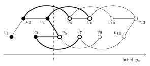
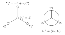
Figure 2: Left: a sweep. The vertices are placed at their labels; the dashed line is the threshold \(t\), the filled vertices form \(S_t\), the thick edges cross the threshold, and the vertices with a thick border form \(\partial^{+}S_t=\{v_5,v_6,v_7,v_8\}\), while \(\partial^{-}S_t=\{v_2,v_3,v_4\}\). Right: the ideal \(3\)-star of Section 2.3. The center \(Z\) and the planar standard Gaussian vector \(G\) are independent, \(w_1,w_2,w_3\) are unit vectors at mutual angles \(\frac{2\pi}3\), and \(s_r=\sqrt{1-r^2}\); the neighbors have correlation \(r\) with the center and sum to \(3rZ\).
2.2 Gaussian labels with critical decay
A vertex lies on a frontier only if one of its edges crosses the threshold, that is, only if the two ends of that edge fall on different sides of it. If two neighbors had equal labels, their edge would never cross. For two standard normal labels with correlation \(\rho\), the probability that they fall on different sides of zero is \(\arccos(\rho)/\pi\) (Sheppard’s formula, Lemma 4.9). So the labels should be as correlated as possible across every edge, while each label keeps unit variance and depends only on a bounded neighborhood, so that labels of far-apart vertices are independent. We take independent standard normal variables \((Z_w)_{w\in V(G)}\) and, for a radius \(R\), with \(B_R(v)=\{w:\mathop{\mathrm{dist}}(v,w)\le R\}\) the ball of radius \(R\) around \(v\), \[\begin{equation*} \tag{2.1} X_v=\sum_{w\in B_R(v)}2^{-\mathop{\mathrm{dist}}(v,w)/2}\,Z_w,\qquad Y_v=X_v/\sqrt{\mathop{\mathrm{Var}}X_v} \end{equation*}\] (Definition 5.2). For maximum degree \(p\) the base \(2\) is replaced by \(p-1\).
Why this choice of weights?
A label is a weighted sum of the variables around the vertex. Normalizing does not change correlations, so it suffices to look at the sums \(X_u,X_v\) of (2.1) for two neighbors \(u,v\). They share the variables \(Z_w\) of every vertex \(w\) in both balls, and the two weights of such a \(Z_w\) differ by a factor at most \(\sqrt2\), because \(\mathop{\mathrm{dist}}(u,w)\) and \(\mathop{\mathrm{dist}}(v,w)\) differ by at most \(1\). Weights with such a bounded ratio give the shared part a correlation at least \(\mathop{\mathrm{sech}}(\frac12\ln2)=\frac{2\sqrt2}3\) (Lemma 5.7); with base \(p-1\) the factor is \(\sqrt{p-1}\) and the bound \(\frac{2\sqrt{p-1}}p\). The only loss comes from the outer shell, the vertices in the ball of \(u\) but not in that of \(v\), and the decay rate decides how much squared mass lies there. If the coefficients decay faster than \(2^{-\mathop{\mathrm{dist}}/2}\), the squared mass sits near the center, each label is close to \(Z_v\) alone, and neighboring labels are nearly independent. If they decay more slowly, the outermost sphere of the ball dominates, and that is where the balls of \(u\) and \(v\) differ. At the critical rate \(2^{-\mathop{\mathrm{dist}}/2}\), every sphere of a tree carries the same squared mass, so the squared mass is spread evenly over the \(R\) layers of the ball, and the outer shell carries only a fraction \(O(1/R)\) of the variance ((5.2)). In a graph that is not a tree the spheres are smaller, which only helps; nothing is assumed about girth, regularity or connectivity.
Lemma (edge correlations; Lemma 5.4). Let \(G\) be a graph with \(\Delta(G)\le3\) and let \((Y_v)\) be the labels (2.1) at radius \(R\). Then every edge \(uv\) satisfies \(\mathop{\mathrm{Corr}}(Y_u,Y_v)\ge r_*(1-\frac1R)\), where \(r_*=\frac{2\sqrt2}3\approx0.9428\). For maximum degree \(p\) and base \(p-1\) the bound is \(\frac{2\sqrt{p-1}}p(1-\frac1R)\).
The constant is best possible for labels whose weights depend only on the distance: on the infinite \(p\)-regular tree, the local limit of \(p\)-regular graphs of large girth, no such radial Gaussian labeling has a neighbor correlation above \(\frac{2\sqrt{p-1}}p\), and the labels approximate the Gaussian wave, which attains this value in the limit (Remark 5.1).
Vertices of degree at most \(2\) can be removed by series–parallel reductions at a cost of \(O(\log n)\) in the pathwidth (Lemma 4.5), so it suffices to bound graphs with \(\delta(G)\ge3\). For such graphs with vertices of several degrees we use mixed labels: a step away from \(v\) through a vertex \(x\) multiplies the coefficient by \((d(x)-1)^{-1/2}\), so that the decay is critical at every vertex at once. An edge whose ends have degrees \(i\) and \(j\) then has correlation at least \(r_{ij}=\mathop{\mathrm{sech}}\bigl(\tfrac14\ln((i-1)(j-1))\bigr)\) up to a factor \(1-o(1)\) (Lemma 5.5); \(r_{33}=r_*\), \(r_{44}=\frac{\sqrt3}2\) and \(r_{55}=\frac45\). For both kinds of labels, \(Y_v\) depends only on the variables in a ball of bounded radius around \(v\), the labels are distinct with probability \(1\), and frontier counts have variance \(O(n)\) (Lemmas 5.6 and 4.10). The radius \(R\) grows slowly with \(n\), so that the loss \(\frac1R\) vanishes while the dependence stays local.
2.3 The star comparison and the simplex theorem
This subsection bounds the probability that a single vertex lies on an outer frontier, using only the correlation bounds of Section 2.2. Summed over the vertices, these bounds give the plain sweep bounds at the end of the subsection, and the median switch and the charging certificate of the next two subsections build on them.
Fix a vertex \(v\) of degree \(d\) with neighbors \(u_1,\dots,u_d\). The vector \((Y_v,Y_{u_1},\dots,Y_{u_d})\) is a centered Gaussian vector with unit variances whose incident correlations \(\mathop{\mathrm{Corr}}(Y_v,Y_{u_i})\), between the center and a neighbor, are at least known lower bounds \(r_i\); we call it a \(d\)-star with lower bounds \(r\) (Definition 6.1), with center \(Y_0=Y_v\) and neighbors \(Y_i=Y_{u_i}\). These lower bounds are all that the labels guarantee. The correlations \(\mathop{\mathrm{Corr}}(Y_i,Y_j)\) between two neighbors are not controlled: short cycles through \(v\) may make them large or small. The vertex lies in \(\partial^{+}S_\tau\) exactly when the frontier event \(\{Y_0>\tau,\ \min_iY_i\le\tau\}\) occurs, and we bound its probability from above in terms of \(r\) alone, in three steps.
Reduction to the center (Lemma 6.2). The first step removes the correlations between neighbors from the problem. The event \(\{Y_0>\tau\}\) is the disjoint union of the frontier event and the event that the whole star lies above \(\tau\). Let \(\Phi\) be the standard normal distribution function. Since \(Y_0\) is standard normal and its distribution is symmetric about \(0\), \(\mathbb{P}(Y_0>\tau)=1-\Phi(\tau)=\Phi(-\tau)\) for every \(\tau\in\mathbb{R}\), positive or negative, and so \[\mathbb{P}\bigl(Y_0>\tau,\ \min_iY_i\le\tau\bigr) =\Phi(-\tau)-\mathbb{P}\bigl(Y_k>\tau\ \text{for}\ 0\le k\le d\bigr).\] It therefore suffices to bound the probability that the whole star lies above \(\tau\) from below. Positively correlated variables tend to exceed a threshold together, so this probability should be smallest when the correlations are smallest. Slepian’s inequality (Slepian 1962) (Lemma 4.8) makes this precise: if two centered Gaussian vectors have the same variances and every covariance of the first is at least the corresponding covariance of the second, then all coordinates of the first exceed \(\tau\) with at least the probability that all coordinates of the second do. So we lower each incident correlation \(\rho_i=\mathop{\mathrm{Corr}}(Y_0,Y_i)\) to exactly \(r_i\), without raising any other correlation. With fresh independent standard normal variables \(\xi_1,\dots,\xi_d\), put \[Y'_0=Y_0,\qquad Y'_i=Y_i-(\rho_i-r_i)\,Y_0+\sqrt{\rho_i^2-r_i^2}\;\xi_i\qquad(1\le i\le d).\] Subtracting a multiple of the center removes the excess correlation with the center, and the noise \(\xi_i\) restores unit variance. A direct computation gives \(\mathop{\mathrm{Var}}Y'_i=1\), \(\mathop{\mathrm{Corr}}(Y'_0,Y'_i)=r_i\) and \(\mathop{\mathrm{Cov}}(Y'_i,Y'_j)=\mathop{\mathrm{Cov}}(Y_i,Y_j)-\rho_i\rho_j+r_ir_j\le\mathop{\mathrm{Cov}}(Y_i,Y_j)\) for \(i\ne j\). So the correlations between neighbors go down as well, whatever they were, and by Slepian’s inequality the new star has at least the frontier probability of the old one.
The new star has a simple structure. Each neighbor is a multiple of the center plus an independent remainder: \(Y'_i=r_iY_0+s_iU_i\), with \(s_i=\sqrt{1-r_i^2}\) and a centered Gaussian vector \(U=(U_1,\dots,U_d)\) with unit variances, independent of \(Y_0\). The incident correlations are now known exactly, and everything unknown about the star sits in the correlation matrix of \(U\). Given \(Y_0=z\), the neighbor \(Y'_i\) lies above \(\tau\) exactly when \(U_i>a_i(z)=(\tau-r_iz)/s_i\). These thresholds decrease as \(z\) grows: a high center pulls its neighbors up. Integrating over the values \(z>\tau\) of the center against its density \(\varphi\), the standard normal density, and taking for each \(z\) the least favorable correlation matrix of \(U\), gives \[\mathbb{P}\bigl(Y_0>\tau,\ \min_iY_i\le\tau\bigr)\ \le\ \Phi(-\tau)-\int_\tau^\infty\varphi(z)\,P_{\min}\bigl(a(z)\bigr)\,dz,\qquad a_i(z)=\frac{\tau-r_iz}{s_i},\] where \(P_{\min}(a)\) is the infimum of \(\mathbb{P}(U_i>a_i\ \forall i)\) over all correlation matrices of \(U\). The right-hand side depends only on \(\tau\) and \(r\), and the next step evaluates \(P_{\min}\).
The simplex theorem (Lemma 6.5). For equal thresholds \(a_1=\dots=a_d=a\) and \(d\le5\) the infimum is attained by the most spread-out configuration, the regular simplex vector \(U^*\): \(d\) standard normal variables with all pairwise correlations \(-\frac1{d-1}\), the most negative common value possible, at which their sum is \(0\). This is a case of a recent theorem of Mulgund (Mulgund 2026), which proves a conjecture of Balitskiy, Karasev and Tsigler (Balitskiy, Karasev, and Tsigler 2017); for three coordinates it also has an elementary proof, and for four it also follows from the four-cap theorem of L. Fejes Tóth (Fejes Tóth 1950; Böröczky 2004). Write \(S_d(a)=\mathbb{P}(U^*_i>a\ \forall i)\).
Ideal stars (Definition 6.7). The first two steps combine into one explicit worst case. Suppose that all lower bounds are equal to some \(r\), as on a \(d\)-regular graph. Then all thresholds \(a_i(z)\) are equal to \((\tau-rz)/s_r\), the simplex theorem gives \(P_{\min}(a(z))=S_d\bigl((\tau-rz)/s_r\bigr)\), and the bound of the first step becomes an explicit integral. This integral is not only a bound: it is the frontier probability of an actual star. Let \(Z\) be standard normal and \(U^*\) the regular simplex vector in \(d\) variables, independent of \(Z\). The ideal \(d\)-star is \(Y^*_0=Z\), \(Y^*_i=rZ+s_rU^*_i\) (Figure 2, right). Its incident correlations are exactly \(r\), and its neighbors are spread out as far as these correlations allow: the remainders \(U^*_i\) sum to \(0\), so the neighbors sum to \(drZ\), and any two neighbors have correlation \(r^2-s_r^2/(d-1)=(dr^2-1)/(d-1)\), the smallest common value possible. Given \(Z=z\), all neighbors lie above \(\tau\) with probability exactly \(S_d\bigl((\tau-rz)/s_r\bigr)\), so the computation of the first step holds with equality for this star. Its frontier probability, the ideal star function, is therefore \[\begin{equation*} \tag{2.2} f_{d,r}(\tau)=\mathbb{P}\bigl(Y^*_0>\tau,\ \min_iY^*_i\le\tau\bigr) =\Phi(-\tau)-\int_\tau^\infty\varphi(z)\,S_d\Bigl(\frac{\tau-rz}{s_r}\Bigr)dz . \end{equation*}\] For \(3\le d\le5\), every \(d\)-star whose lower bounds are all at least \(r\) has frontier probability at most \(f_{d,r}(\tau)\) at every threshold \(\tau\), and so does every star with fewer than \(d\) neighbors and such lower bounds, because adding neighbors can only enlarge the frontier event (Corollary 6.8). As the ideal star is itself a \(d\)-star with lower bounds \(r\), no better bound follows from the lower bounds alone.
The layout lemma takes the largest frontier over all thresholds, so what counts is the worst threshold. The suprema \[F_3=\sup_\tau f_{3,r_{33}}(\tau)\approx0.1401583,\qquad F_4=\sup_\tau f_{4,r_{44}}(\tau)\approx0.2457720\] are enclosed rigorously in ball arithmetic (Proposition 6.9); the first is attained near \(\tau\approx-0.068\), the second near \(\tau\approx-0.164\). For a graph of maximum degree \(4\), the labels with base \(3\) give every edge correlation at least \(r_{44}(1-\frac1R)\), so every vertex lies in \(\partial^{+}S_\tau\) with probability at most \(f_{4,r_{44}}(\tau)+o(1)\le F_4+o(1)\). By linearity of expectation, \(\mathbb{E}|\partial^{+}S_\tau|\le F_4n+o(n)\) at every threshold, and concentration, the finite grid of thresholds and the layout lemma turn this into a bound on the pathwidth. For maximum degree \(3\) the same argument with the labels (2.1) gives \(F_3\). This is the plain sweep, the layout lemma applied to the Gaussian labels.
Theorem (plain sweep; Theorem 7.1(a) and the case \(n_4=0\) of Theorem 7.1(b)). Every graph with \(\Delta(G)\le4\) satisfies \(\mathop{\mathrm{pw}}(G)\le F_4n+o(n)\), and every graph with \(\Delta(G)\le3\) satisfies \(\mathop{\mathrm{pw}}(G)\le F_3n+o(n)\).
This is where the plain sweep stops. For maximum degree \(3\), the coefficient \(F_3\) is the best that any analysis of the outer frontiers can give, because it is essentially attained: on cubic graphs of large girth the stars of the labels are nearly ideal, so the outer frontier at the threshold \(\tau\approx-0.068\) has about \(F_3n\) vertices. Improving the bound requires changing the layout, not the analysis.
2.4 The median switch
The change is suggested by the shape of \(f_{3,r}\) (Figure 1). At the median threshold \(0\) its value has a closed form. Since \(Y^*_1+Y^*_2+Y^*_3=3rY^*_0\), all three neighbors can be positive only when the center is. So \(f_{3,r}(0)\) is one half minus the probability that three standard normal variables with pairwise correlation \(b(r)=\frac{3r^2-1}2\) are all positive, and Sheppard’s formula gives \[\begin{equation*} \tag{2.3} f_{3,r}(0)=\kappa(r):=\frac3{4\pi}\arccos\frac{3r^2-1}2,\qquad \kappa(r_*)=\frac3{4\pi}\arccos\frac56=c_{3} \end{equation*}\] (Lemma 8.6). Moreover \(f_{3,r}(t)\le f_{3,r}(0)\) for every \(t\ge0\) (Lemma 8.7). So \(f_{3,r}\) exceeds its value at the median only below the median, and there we use the inner frontier instead. Since \(-Y\) has the same distribution as \(Y\) (sign symmetry), the event \(v\in\partial^{-}S_t\) for \(Y\) is the event \(v\in\partial^{+}S_{-t}\) for \(-Y\), whose probability is at most \(f_{3,r}(-t)\le\kappa(r)\) when \(t\le0\) (Proposition 8.8). A layout with inner frontiers below zero and outer frontiers above zero therefore has expected frontier size at most \(\kappa(r)n\) at every nonzero threshold.
The difficulty lies at threshold zero, where the layout must pass from the inner frontier \(U=\partial^{-}S_0\) to the outer frontier \(W=\partial^{+}S_0\) while every edge between \(S_0\) and its complement stays covered. Putting \(U\cup W\) into one bag would give a bag of about \(2\kappa(r)n\) vertices. The connector does better: it adds the vertices of \(W\) one at a time, in an order given by a purely combinatorial lemma (Lemma 8.3), and drops a vertex of \(U\) as soon as all its neighbors above zero are present. Only the vertices whose three neighbors all lie on the other side of zero obstruct this exchange; let \(D\) be their set.
Lemma (median-switched layout; Lemma 8.4). Let \(\Delta(G)\le3\) and let \(y\) be an injective labeling. If \(|\partial^{-}S_t|\le w\) for all \(t<0\), \(|\partial^{+}S_t|\le w\) for all \(t>0\), and \(\max\bigl(|U|+|D\cap W|,\ |W|+|D\cap U|\bigr)+1\le w\), then \(\mathop{\mathrm{pw}}(G)\le w\).
For a vertex \(v\) of degree \(d\le3\), the events \(v\in U\) and \(v\in D\cap W\) are \(\{Y_v\le0<\max_iY_{u_i}\}\) and \(\{d=3,\ Y_v>0\ge\max_iY_{u_i}\}\). The connector adds nothing at leading order because of the following lemma, whose right side is the same bound \(\kappa(r)\) as at nonzero thresholds.
Lemma (switch lemma; Lemma 8.9). Let \((Y_0,Y_1,\dots,Y_d)\) be a \(d\)-star with all lower bounds equal to \(r\in(0,1)\) and \(d\le3\). Then \[\mathbb{P}\bigl(Y_0\le0,\ \exists i:\ Y_i>0\bigr) +\mathbf{1}_{d=3}\mathbb{P}\bigl(Y_0>0,\ Y_i\le0\text{ for all }i\bigr)\ \le\ \kappa(r).\]
At the ideal star the second event is impossible, since the neighbor labels sum to \(3r\) times the center label, and the first has probability exactly \(\kappa(r)\); a star that makes the second event possible loses at least as much in the first. After conditioning on the center, the proof reduces to showing that the probability that at least two of three standard normal residuals exceed a level \(h>0\) is smallest for the equilateral matrix of \(U^*\) (Lemma 8.11). This is not an orthant event, so Slepian’s inequality does not apply; a deformation monitored by Plackett’s identity (Lemma 4.7) reduces it to the planar case. Concentration and \(R\to\infty\) then give the bound with constant \(\kappa(r_*)=c_{3}\).
Theorem (Theorem 8.1). Every graph \(G\) with \(\Delta(G)\le3\) satisfies \(\mathop{\mathrm{pw}}(G)\le c_{3}\,n+o(n)\).
The gain over the plain sweep is small, \(F_3-c_{3}\approx3.4\cdot10^{-4}\). But the median switch replaces a numerically enclosed maximum by a closed form, and its proof uses no computation. The value \(c_{3}\) is exactly what the median-switched sweep gives on cubic graphs of large girth, so any further improvement must change the rule at threshold zero (Section 15). With mixed labels, the same layout gives Theorem 8.2.
2.5 Mixed degrees, the charging certificate and the bootstrap
Degrees 3 to 5.
With mixed labels, the lower bounds \(r_{d(v)d(u)}\) of the star of \(v\) depend on the degrees of its neighbors. So the bound of the reduction to the center depends on the type \(T=(d;k_3,k_4,k_5)\) of \(v\), where \(d\) is its degree and \(k_j\) counts its neighbors of degree \(j\). We write this bound \(C_T(\tau)\); there are \(46\) types for degrees \(3\) to \(5\) (Definition 7.3). A vertex of degree \(3\) next to vertices of higher degree has weaker correlations than one in a cubic region, and its bound exceeds the coefficient \(a_3\) that we aim for. We move the excess along the edges: a vertex of degree \(i\) sends an amount \(t_{ij}\) along each edge to a neighbor of degree \(j>i\). The transfers sum to zero over the graph (Lemma 7.4). Hence \(\mathbb{E}|\partial^{+}S_\tau|\le\sum_da_dn_d\) whenever \((a_3,a_4,a_5)\) is admissible, that is, whenever for every \(\tau\in[-3,3]\) some transfer vector \((t_{34},t_{35},t_{45})\) brings the transferred bound of every type below the coefficient of its degree. (Beyond \(|\tau|=3\) the frontier probabilities are below \(5\Phi(-3)<0.007\).)
We verify admissibility by a computer-assisted proof (Proposition 7.5). The thresholds are partitioned into cells. Each cell has one transfer vector and, for every type, a rational lower bound on the integral in \(C_T(\tau)\), obtained in ball arithmetic. The final inequalities are checked in exact rational arithmetic with positive slack. This certifies the pathwidth sequences \[\mathsf{P}=(F_3,\,0.2575,\,0.3667),\qquad \mathsf{R}=(0.1455,\,0.2530,\,0.3600),\qquad \mathsf{S}=\bigl(\tfrac5{32},\,\tfrac14,\,\tfrac{11}{32}\bigr)\] of Theorem 7.2; the bounds \((F_3,0.2575)\) and \((\frac5{32},\frac14)\) for maximum degree \(4\) (Theorem 7.1(b),(c)) are their restrictions to graphs without vertices of degree \(5\). The triple \(\mathsf{P}\) is best when few vertices have degree \(4\) or \(5\), \(\mathsf{S}\) when many do. All coefficient vectors of the paper are collected in Theorem 9.2.
All graphs.
Beyond degree \(5\) no probability is involved. A combinatorial induction in the spirit of Fomin, Gaspers, Saurabh and Stepanov (Fomin et al. 2009) and of Edwards and McDermid (Edwards and McDermid 2015) deletes vertices of large degree one at a time (Proposition 9.10). Putting a deleted vertex back into every bag adds at most one to the width, and we compare this increase with the decrease of the potential \(\sum_vb_{d(v)}\). Deleting a vertex \(w\) of maximum degree \(d\) removes the term \(b_d\) of \(w\) itself. It also lowers the degree of each neighbor by one, which lowers the potential by an increment \(h_{d'}=b_{d'}-b_{d'-1}\), where \(d'\) is the degree of the neighbor; this increment is at least the running minimum \(H_d=\min_{3\le i\le d}h_i\). With \(d-1\) neighbors of degree \(d\) and one of smaller degree, the decrease balances the increase exactly when \(1-b_d=(d-1)H_d+H_{d-1}\), and the two worst cases give the recurrence \[\begin{equation*} \tag{2.4} b_d=\max\Bigl\{\frac{1+(d-1)\,b_{d-1}-H_{d-1}}{d},\;1-d\,H_{d-1}\Bigr\}\qquad(d>k) \end{equation*}\] ((9.1)). Vertices of degree at most \(2\) are removed by the classical series–parallel reductions after every deletion, and all reductions together add \(O(\log n)\) to the pathwidth (Lemma 4.5).
The bootstrap lemma (Lemma 9.3) gives the coefficients \(b_d\) for \(d>k\) from a base of maximum degree \(k\) by (2.4). When the increments are nonincreasing, the first term of the maximum is the larger one, and (2.4) is the recurrence \(d\,b_d=(d-2)\,b_{d-1}+b_{d-2}+1\) of Edwards and McDermid (Remark 9.4). The recurrence also explains why a better cubic constant alone improves nothing at higher degrees: with \(k=3\) and \(b_3=c_{3}<\frac16\) the second term is the larger one, and \(b_4=1-4c_{3}\approx0.4407\), worse than the known \(\frac13\). Theorem 1.3 is therefore bootstrapped from the degree-\(5\) base \(\mathsf{S}\): its coefficients are \(\frac{3d-4}{32}\) up to degree \(6\), then \(1-\frac{111}{28(d+1)}\) up to degree \(10\) and \(1-\frac4{d+1}\) from degree \(11\) on. The edge bound follows because \(2a_d/d\le\frac7{48}\) for every \(d\), with equality only at \(d=6\), where \(a_6=\frac7{16}\) (Corollary 1.4); applying this to every component separately also gives a remainder \(o(m)\) (Remark 9.14).
2.6 Algorithms and running times
Section 10 turns the existence proofs into algorithms. It replaces the Gaussian variables by a finite rational distribution coupled to the normal distribution, which changes every per-vertex probability of Part I by \(o(1)\) uniformly in the threshold (Lemmas A.23 and A.24), and then fixes the variables one at a time by the method of conditional expectations (Erdős and Selfridge 1973; Raghavan 1988), applied to finitely many local counts (Lemma A.27). The radius grows only like \(\frac18\log_2\log_2n\), so each conditional expectation is computable by local enumeration in \(n^{o(1)}\) time.
Part II turns the widths into running times in three ways. Substitution: a dynamic program with \(c^{w+1}\mathop{\mathrm{poly}}(n)\) steps over a path decomposition of width \(W(G)+o(n)\) runs in time \(c^{W(G)+o(n)}\mathop{\mathrm{poly}}(n)\) (Lemma 11.1); this gives most bounds of Section 11 and, through Cut&Count, the rank-based approach and algorithms over orderings of small cutwidth, those of Section 14. Rerunning a measure-and-conquer analysis: in polynomial space the widths enter Separate, Measure and Conquer (Gaspers and Sorkin 2017) through balanced separators of size \(cn\), and the separator constant enters the mathematical program of the analysis in one or two places (Lemma C.5, Theorem C.3). Moving a switch point: with coefficient \(\frac14\) in place of \(\frac13\) at degree \(4\), the algorithm of Nederlof, van Rooij and van Dijk (Nederlof, Rooij, and Dijk 2014) for counting dominating sets can hand the sets of size \(4\) to its dynamic program, which lowers its running time from \(1.5002^n\) to \(1.4815^n\) (Theorem 13.1).
Table 2: Running-time bounds of this paper that, as far as we know, the preprints (OpenAI 2026b; Claude 2026) that claim to refute ETH do not affect (Section 1.2). Letters refer to the notes that follow the table.
| Problem | Previous | New | References |
|---|---|---|---|
| Feedback vertex sets | |||
| Feedback Vertex Set, | {n/3}<1.2600n | f, Thm. 14.1 | |
| Feedback Vertex Set, , det. | {F_4n}<1.4853n | , Thm. 14.1 | |
| Feedback Vertex Set, | {0.5121n}<1.4262n | f, Thm. 14.1 | |
| Feedback Vertex Set, | {7n/16}<1.6172n | f, Thm. 14.1 | |
| Connected FVS and otherse, | {c_{3}n}<1.2139n | f, Thm. 14.1 | |
| Connected FVS and otherse, | {F_4n}<1.4060n | f, Thm. 14.1 | |
| Connected FVS and otherse, | {11n/32}<1.6105n | f, Thm. 14.1 | |
| Domination | |||
| (#)Min. Weight Dominating Setc | a, Thm. 13.1 | ||
| (#)Min. Weight Dominating Set, | {n/6}<1.2010n | {c_{3}n}<1.1661n | , Thm. 11.4 |
| Connected Dominating Set, | {c_{3}n}<1.1661n | f, Thm. 14.1 | |
| Connected Dominating Set, | {F_4n}<1.4060n | f, Thm. 14.1 | |
| Connected Dominating Set, | {11n/32}<1.6105n | , Thm. 14.1 | |
| Independence and vertex covers | |||
| (#)Max. Weight Indep. Set, | {n/6}<1.1225n | {c_{3}n}<1.1018n | , Thm. 11.4 |
| (#)Max. Weight Indep. Set, | {n/3}<1.2600n | {F_4n}<1.1858n | , Thm. 11.4 |
| Connected Vertex Cover, | {n/3}<1.2600n | f, Thm. 14.1 | |
| Connected Vertex Cover, | {0.5121n}<1.4262n | f, Thm. 14.1 | |
| Max 2-CSP | |||
| Max -CSP, all instances | {13m/75}<r{m/5.769} | {7m/48}<r{m/6.857} | , Thm. 11.3 |
| Max -CSP, | {c_{3}n}<r{0.13983n} | , Thm. 11.3 | |
| Max -CSP, | , | , | , , Thm. 11.3 |
| Max -CSPb, avg. degree | {n(1-3.5/(d+1)+O(d{-3}))} | , Thm. 11.3 | |
| Max -CSPb, avg. degree | {n(1-3.5/(d+1)+O(d{-3}))} | , Thm. 11.3 | |
| Patterns and packings | |||
| Counting -edge subgraphsd | {(7/48)k}<n{0.1459k} | , Thm. 11.5 | |
| Counting -paths, -cyclesd | , Thm. 11.5 | ||
| Permutation Pattern Matching | {O(k)}n{(253/1215)k} | , Thm. 11.8 | |
| -opt for TSP, general graphs | , Thm. 11.8 | ||
| -opt for TSP, bounded degree | , Thm. 11.8 | ||
| Co-Path Packing | , Thm. 14.1 | ||
| -Co-Path Set | , Thm. 14.1 | ||
| Cycles and paths | |||
| Hamiltonian Cycle, | f, Thm. 14.1 | ||
| Hamiltonian Cycle, | f,g, Thm. 14.1 | ||
| Hamiltonian Cycle, | f, Thm. 14.1 | ||
| Hamiltonian Cycle, avg. degree | , Thm. 14.1 | ||
| TSP, , det. | , Thm. 14.1 | ||
| TSP, , det. | g, Thm. 14.1 | ||
| TSP, , det. | g, Thm. 14.1 | ||
| TSP, , det. | , Thm. 14.1 | ||
| TSP, avg. degree , det. | , Thm. 14.1 | ||
| Longest Path, | f, Thm. 14.1 | ||
| Longest Path, | f, Thm. 14.1 | ||
| Longest Path, | f, Thm. 14.1 | ||
| Other connectivity problems | |||
| Steiner Tree, | {c_{3}n}<1.1661n | f, Thm. 14.1 | |
| Steiner Tree, | {F_4n}<1.3100n | , Thm. 14.1 | |
| Max Internal Spanning Tree, | {7n/16}<1.8341n | f, Thm. 14.1 | |
| Directed problems | |||
| Directed problemsh, | {c_{3}n}<1.2848n | f, Thm. 14.1 | |
| Directed problemsh, | {F_4n}<1.5533n | f, Thm. 14.1 | |
Notes to Table 2.
A letter after a citation concerns the previous bound, and a letter after a problem concerns the whole row. a A gap in the analysis of this algorithm allowed us only to reconstruct a running time of \(O(1.5004^n)\) (Appendix D.5). b A record only for moderate \(\bar d\); for large \(\bar d\), the algorithms of Williams (Williams 2005), for integer scores of polynomial size, and of Golovnev and Kutzkov (Golovnev and Kutzkov 2014), for Boolean domains, are faster (Theorem 11.3). c When the set of possible weight sums has polynomial size, as in (Nederlof, Rooij, and Dijk 2014 Cor. 32) (minimum weight) and (Rooij 2011 Cor. 8.14) (counting). d Both bounds carry a further factor \(k^{O(k)}\). e The problems of Theorem 14.1(b) other than Connected Dominating Set: Connected Feedback Vertex Set, Connected Odd Cycle Transversal, Exact \(k\)-Leaf Spanning Tree, Maximum Full Degree Spanning Tree, Graph Metric Traveling Salesperson, and undirected Min Cycle Cover and Longest Cycle; Maximum Leaf Spanning Tree also has the bounds of Connected Dominating Set. f By a Monte Carlo algorithm. g The cited algorithm, run with the pathwidth bounds of (Fomin et al. 2009), and for TSP with \(\omega\le\frac94\). h The directed versions of Min Cycle Cover, Longest Path and Longest Cycle, and Exact \(k\)-Leaf Outbranching; \(\Delta\) is the maximum degree of the underlying undirected graph.
The bounds for TSP, previous and new, are evaluated with the matrix multiplication exponent \(\omega\le\frac94\) (OpenAI 2026a; Amanov, Berg, and Zuiddam 2026) (Section 14).