Appendix A Deferred proofs

This appendix collects the proofs deferred from the main text. The first five subsections restate the deferred statements, with their numbers in the main text, and prove them: Lemma 4.5 in Appendix A.1; Proposition 6.9 and the tools of the certificate behind Proposition 7.5 in Appendix A.2; Theorem 8.2 in Appendix A.3; Theorem 9.2 and Corollary 9.5 in Appendix A.4; and Theorem 10.1, Corollary 10.2 and Theorem 10.3 in Appendix A.5. The next, Appendix A.6, restates nothing: it completes the proof of Theorem 10.1 in the cases that use the median-switched layout. The last, Appendix A.7, proves Lemmas 11.2, 11.6 and 11.7 and Theorems 11.8 and 14.1 of Part II; the analyses behind Theorems C.3, C.6 and 13.1 have appendices of their own (Appendices C and D).

A.1 Proof of the reduction lemma

This subsection proves Lemma 4.5, with the reduction operations of Definition 4.2, their properties (RP1)–(RP3) and the two facts Lemmas 4.3 and 4.4 of Section 4.3.

Lemma 4.5 (undoing reductions; restated). Let \(F\) be a nonempty graph. Apply to \(F\) any finite sequence of steps, each of which is a reduction operation or the deletion of a vertex of the current graph. Let \(D\) be the set of vertices removed by deletions and \(R\) the final graph. Then:

(a)  \(\mathop{\mathrm{pw}}(F)\le|D|+\mathop{\mathrm{pw}}(R)+3\log_2|V(F)|+1\);

(b)  every edge of \(F-D\) with both ends in \(V(R)\) is an edge of \(R\), and for every component \(C\) of \((F-D)-V(R)\), the set \(N_{F-D}(C)\) is empty, a single vertex, or the two ends of an edge of \(R\), and \(\mathop{\mathrm{tw}}(F[C])\le2\).

Proof. The proof follows the sequence step by step. The vertices removed so far by reductions induce components in \(F\) minus the vertices deleted so far. We maintain as an invariant that each of these components has treewidth at most \(2\) and attaches to the current graph at no vertex, at one vertex, or at the two ends of an edge. At the end, a path decomposition of the final graph \(R\) is extended to one of \(F-D\) by inserting path decompositions of these components, each of width at most \(3\log_2|V(F)|\) by Lemma 4.4, next to bags that contain their attachments. Adding \(D\) to every bag then gives the claim.

The invariants. Write \(n=|V(F)|\). Let \(H_t\) be the current graph after \(t\) steps, \(D_t\) the set of vertices deleted in the first \(t\) steps, and \(F_t:=F-D_t\). Then \(V(H_t)\subseteq V(F_t)\), but \(H_t\) need not be a subgraph of \(F_t\), since (R3) adds edges. For a component \(C\) of \(F_t-V(H_t)\) put \(S_C:=N_{F_t}(C)\); these are vertices of \(H_t\). We maintain two invariants:

(I1)  every edge of \(F_t\) with both ends in \(V(H_t)\) is an edge of \(H_t\);

(I2)  for every component \(C\) of \(F_t-V(H_t)\): \(|S_C|\le2\); if \(|S_C|=2\) then \(S_C\) spans an edge of \(H_t\); and the graph \(Q^+_C\) obtained from \(Q_C:=F_t[C\cup S_C]\) by adding the edge on \(S_C\) when \(|S_C|=2\) has treewidth at most \(2\).

Both hold for \(t=0\), when \(H_0=F_0=F\) and there are no components.

A deletion of a vertex \(w\in V(H_t)\) removes \(w\) from both graphs. Edges of \(F_{t+1}\) inside \(V(H_{t+1})\) are edges of \(F_t\) inside \(V(H_t)\) avoiding \(w\), hence edges of \(H_t-w=H_{t+1}\); so (I1) holds. The graph \(F_t-V(H_t)\) does not change, each \(S_C\) loses at most the vertex \(w\), an edge on \(S_C\) that avoids \(w\) survives in \(H_{t+1}\), and each new \(Q^+_C\) is a subgraph of the old one. So (I2) holds.

A reduction operation at a vertex \(v\). Let \(N:=N_{H_t}(v)\), so \(|N|\le2\). Here \(F_{t+1}=F_t\) and \(V(H_{t+1})=V(H_t)\setminus\{v\}\). Edges of \(F_t\) inside \(V(H_{t+1})\) are edges of \(H_t\) not incident with \(v\), and these survive in \(H_{t+1}\); so (I1) holds. The components \(C\) of \(F_t-V(H_t)\) with \(v\notin S_C\) remain components, with the same \(S_C\), the same \(Q^+_C\), and an edge on \(S_C\) that avoids \(v\) and therefore survives. The components \(C\) with \(v\in S_C\) merge with \(v\) into one new component \(C'\). We check (I2) for \(C'\).

• \(S_{C'}\subseteq N\). A neighbor of \(v\) in \(F_t\) outside \(C'\) lies in \(V(H_t)\), so by (I1) it lies in \(N\). A neighbor of a merged \(C\) outside \(C'\) lies in \(S_C\setminus\{v\}\); if this set is nonempty, \(S_C=\{v,u\}\) spans an edge of \(H_t\) by (I2), so \(u\in N\).

• If \(|S_{C'}|=2\), then \(N=S_{C'}=\{x,y\}\), so \(v\) had degree \(2\) and the operation was (R3) or (R4). In both cases \(xy\in E(H_{t+1})\).

• Let \(K\) be the graph on \(\{v\}\cup N\) with the edges from \(v\) to \(N\), and with the edge \(xy\) if \(N=\{x,y\}\); it has at most three vertices, so \(\mathop{\mathrm{tw}}(K)\le2\). Every edge of \(Q_{C'}=F_t[C'\cup S_{C'}]\) lies in \(K\) or in some \(Q_C\) with \(C\) merged: edges at \(v\) go to \(N\) or into some merged \(C\); edges at a vertex of a merged \(C\) stay in \(C\cup S_C\); and an edge inside \(S_{C'}\) exists only if \(S_{C'}=N=\{x,y\}\), in which case it is the edge \(xy\) of \(K\). The added edge on \(S_{C'}\) (if \(|S_{C'}|=2\)) is also an edge of \(K\). Hence \(Q^+_{C'}\) is a subgraph of the union of \(K\) and the graphs \(Q^+_C\) for the merged \(C\). Each \(Q^+_C\) meets \(K\) exactly in \(S_C\) (the set \(C\) is disjoint from \(V(H_t)\supseteq\{v\}\cup N\), and \(S_C\subseteq\{v\}\cup N\) by the first item), and different \(Q^+_C\) meet only inside \(K\). Each \(S_C\) is the vertex \(v\) or an edge \(vu\) with \(u\in N\), which is an edge of both \(K\) and \(Q^+_C\). Gluing the graphs \(Q^+_C\) to \(K\) one at a time, Lemma 4.3 gives \(\mathop{\mathrm{tw}}(Q^+_{C'})\le2\).

The final decomposition. At the end, \(H_T=R\) and \(F_T=F-D\). Every component \(C\) of \((F-D)-V(R)\) induces a graph \(F[C]\subseteq Q^+_C\) of treewidth at most \(2\) on at most \(n\) vertices, so \(\mathop{\mathrm{pw}}(F[C])\le3\log_2n\) by Lemma 4.4. Take a path decomposition \(W_1,\dots,W_s\) of \(R\) of width \(\mathop{\mathrm{pw}}(R)\) (no bags if \(R\) is empty). For each \(C\) with \(S_C\ne\emptyset\) choose \(i\) with \(S_C\subseteq W_i\), which is possible because \(S_C\) is a vertex or spans an edge of \(R\) by (I2). Immediately after \(W_i\) insert the bags \(W_i\cup P\) for the bags \(P\) of a path decomposition of \(F[C]\) of minimum width, the components assigned to the same \(i\) one after another. Append the path decompositions of the components with \(S_C=\emptyset\) at the end. The result is a path decomposition of \(F-D\):

• every edge inside \(V(R)\) is an edge of \(R\) by (I1) and lies in some \(W_i\); every other edge has an end in some \(C\) and its other end in \(C\cup S_C\), so it lies in an inserted bag \(W_i\cup P\) or in a bag of \(F[C]\);

• a vertex of \(C\) occurs only in the consecutive bags inserted for \(C\);

• a vertex \(x\in V(R)\) occurs in a consecutive run of the bags \(W_i\), and every bag inserted after \(W_i\) contains \(W_i\); so \(x\) occurs in the bags inserted after \(W_i\) exactly when \(x\in W_i\), and its bags remain consecutive.

Every bag has at most \((\mathop{\mathrm{pw}}(R)+1)+(3\log_2n+1)\) vertices, so \(\mathop{\mathrm{pw}}(F-D)\le\mathop{\mathrm{pw}}(R)+3\log_2n+1\); this also holds when \(R\) is empty, since then \(\mathop{\mathrm{pw}}(R)=-1\). Adding \(D\) to every bag gives \(\mathop{\mathrm{pw}}(F)\le|D|+\mathop{\mathrm{pw}}(R)+3\log_2n+1\), which implies (a).

Part (b) is (I1) and (I2) for \(t=T\), since \(H_T=R\), \(F_T=F-D\), \(S_C=N_{F-D}(C)\) and \(F[C]\subseteq Q^+_C\).  ∎

A.2 The star-bound certificate

This subsection describes the computer-assisted proof of Proposition 7.5: the triples \(\mathsf{P},\mathsf{R},\mathsf{S}\) are admissible for \(D=\{3,4,5\}\) (Definition 7.3). Admissibility asks that for every threshold \(\tau\in[-3,3]\) there is a transfer vector \(t\) such that, for every type \(T\) of degree \(d\), the reference star bound \(C_T(\tau)\) plus the transfer term \(\lambda_T(t)\) is at most the coefficient \(a_d\). The certificate replaces the continuum of thresholds by finitely many cells. It bounds each reference star bound from above through a lower Riemann sum of explicit lower bounds for the orthant infimum \(P_{\min}\) of Section 6. The code also certifies the pair \((F_3,0.2575)\) for \(D=\{3,4\}\) directly, although its admissibility follows from that of \(\mathsf{P}\) by restriction to \(D=\{3,4\}\).

Appendices A.2.1 and A.2.2 collect the tools of the star bounds that the certificate uses and prove the enclosures of \(F_3\) and \(F_4\). Appendix A.2.3 proves that the replacement by cells and sums is valid. Appendix A.2.4 describes the rigorous arithmetic, Appendix A.2.5 the search for cells and the results, Appendix A.2.6 how the runs are reproduced, and Appendix A.2.7 what is trusted.

A.2.1 Tools from the star bounds

This subsection collects the lower bounds on \(P_{\min}\) for unequal thresholds and the recursion for the simplex orthant that the certificate and Appendix A.2.2 use; the notation is that of Section 6.

Unequal thresholds.

When the lower bounds \(r_i\) of a star differ, the thresholds \(a_i(z)=(\tau-r_iz)/s_i\) of the center bound differ, and the simplex theorem (Lemma 6.5) does not apply directly. The certificate of Appendix A.2 uses the following two lower bounds on the infimum \(P_{\min}\). The first holds for every \(d\in\{3,4,5\}\) and is exact for equal thresholds; the second is specific to \(d=3\) and is much sharper for unequal thresholds. For \(d\in\{3,4,5\}\) and \(a\in\mathbb{R}^d\) put \[\Lambda_d(a):=\max\Bigl\{0,\ 1-\sum_i\Phi(a_i),\ \max_{1\le j\le d}\Bigl(S_d(a_j)-\sum_{i:\,a_i>a_j}\bigl(\Phi(a_i)-\Phi(a_j)\bigr)\Bigr)\Bigr\}.\]

Lemma A.1 (simplex truncation).  Let \(d\in\{3,4,5\}\) and \(a\in\mathbb{R}^d\). Then \(P^{(d)}_{\min}(a)\ge\Lambda_d(a)\).

Proof. Let \(U\) be a centered Gaussian vector in \(\mathbb{R}^d\) with unit variances. The probability \(\mathbb{P}(U_i>a_i\ \forall i)\) is nonnegative, and it is at least \(1-\sum_i\Phi(a_i)\) by the union bound \(\mathbb{P}(\exists i:\ U_i\le a_i)\le\sum_i\Phi(a_i)\). Let \(\lambda\in\mathbb{R}\). If \(U_i>\lambda\) for all \(i\) but \(U_k\le a_k\) for some \(k\), then \(\lambda<U_k\le a_k\), so in particular \(a_k>\lambda\). Hence \[\{U_i>\lambda\ \forall i\}\ \subseteq\ \{U_i>a_i\ \forall i\}\ \cup \bigcup_{k:\,a_k>\lambda}\{\lambda<U_k\le a_k\},\] and \(\mathbb{P}(\lambda<U_k\le a_k)=\Phi(a_k)-\Phi(\lambda)\). With \(\mathbb{P}(U_i>\lambda\ \forall i)\ge S_d(\lambda)\) from Lemma 6.5, this gives \[\mathbb{P}(U_i>a_i\ \forall i)\ \ge\ S_d(\lambda)-\sum_{i:\,a_i>\lambda}\bigl(\Phi(a_i)-\Phi(\lambda)\bigr).\] Taking \(\lambda=a_j\) for each \(j\) and then the infimum over \(U\) gives \(P^{(d)}_{\min}(a)\ge\Lambda_d(a)\).  ∎

For equal thresholds the bound is exact: every sum over \(\{i:a_i>a_j\}\) is empty, and \(S_d(a)\ge\max\{0,1-d\,\Phi(a)\}\) by the union bound applied to \(U^*\), so \(\Lambda_d(a,\dots,a)=S_d(a)=P^{(d)}_{\min}(a,\dots,a)\) by Lemma 6.5.

For three variables, the rank reduction of Lemma 6.4, which allows unequal thresholds, leads to a planar picture that can be counted exactly. The following bound is used for the stars of a degree-\(3\) vertex whose neighbors do not all have the same degree.

Lemma A.2 (rank reduction and arc count, \(d=3\)).  Let \(a\in\mathbb{R}^3\). For \(\rho>0\) put \(\gamma_i(\rho)=\arccos\mathop{\mathrm{clip}}(-a_i/\rho,-1,1)\in[0,\pi]\), where \(\mathop{\mathrm{clip}}(x,-1,1)=\max\{-1,\min\{1,x\}\}\). Then for all \(0\le\rho_a\le\rho_b\), \[P^{(3)}_{\min}(a)\ \ge\ \int_{\rho_a}^{\rho_b}\Bigl(1-\sum_{i=1}^3\frac{\gamma_i(\rho)}{\pi}\Bigr)\rho\,e^{-\rho^2/2}\,d\rho .\]

Proof. Let \(U\) be a centered Gaussian vector in \(\mathbb{R}^3\) with unit variances and correlation matrix \(C\).

Rank reduction. By Lemma 6.4 it suffices to bound \(\mathbb{P}(U_i>a_i\ \forall i)\) from below when \(C\) is singular, that is, \(\operatorname{rank}C\le2\). Then \(U\) has the distribution of \((\langle v_i,G\rangle)_i\) for unit vectors \(v_1,v_2,v_3\in\mathbb{R}^2\) and a standard Gaussian vector \(G\) in \(\mathbb{R}^2\).

Arc count. Write \(G=\rho(\cos\vartheta,\sin\vartheta)\), so \(\rho\) has density \(\rho e^{-\rho^2/2}\) on \((0,\infty)\) and \(\vartheta\) is uniform and independent of \(\rho\). Given \(\rho>0\), the event \(\{U_i\le a_i\}\) says \(\langle-v_i,(\cos\vartheta,\sin\vartheta)\rangle\ge-a_i/\rho\). If \(-a_i/\rho>1\) this set of directions is empty, if \(-a_i/\rho<-1\) it is the whole circle, and otherwise it is a closed arc of half-angle \(\arccos(-a_i/\rho)\) around the direction of \(-v_i\). In all three cases its normalized length is \(\gamma_i(\rho)/\pi\) (up to a null set). By the union bound, the conditional probability of \(\{U_i>a_i\ \forall i\}\) given \(\rho\) is at least \(\max\{0,1-\sum_i\gamma_i(\rho)/\pi\}\). Integrating against the density of \(\rho\), and dropping the nonnegative contribution of \(\rho\notin[\rho_a,\rho_b]\), \[\mathbb{P}(U_i>a_i\ \forall i)\ \ge\ \int_{\rho_a}^{\rho_b}\Bigl(1-\sum_i\frac{\gamma_i(\rho)}{\pi}\Bigr)\rho e^{-\rho^2/2}\,d\rho .\] The right side does not depend on \(U\), so it also bounds the infimum \(P_{\min}(a)\).  ∎

The interval \([\rho_a,\rho_b]\) is a free parameter; any choice gives a valid bound. The certificate takes \(\rho_a=\max\{0,a_1,a_2,a_3\}\), below which some \(\gamma_i=\pi\) and the integrand is negative, and \(\rho_b\) close to the first zero of the integrand beyond \(\rho_a\). The integral has a closed form in terms of Owen’s \(T\) function (Lemma A.8).

Evaluating the simplex orthant.

The functions \(S_d\) are evaluated through the reflection \(T_d(h)=S_d(-h)\), the distribution function of the maximum of the regular simplex vector. It satisfies a one-dimensional recursion in \(d\), which is the basis of all numerical evaluations of \(S_3,S_4,S_5\) in this paper.

Lemma A.3 (simplex recursion).  For \(h\ge0\), \(T_2(h)=2\Phi(h)-1\), and for \(d\ge3\), \[T_d(h)=\int_0^h d\,\varphi(x)\,T_{d-1}\Bigl(\sqrt{\tfrac d{d-2}}\;x\Bigr)\,dx ;\] for \(h\le0\), \(T_d(h)=0\). In particular each \(T_d\) is continuous and nondecreasing, and \(S_d(a)=T_d(-a)\) is continuous and nonincreasing.

Proof. Let \(X=U^*\) be the regular simplex vector in \(d\) variables. For \(d=2\) we have \(X_2=-X_1\) (the correlation is \(-1\)), so \(\max_iX_i=|X_1|\) and \(T_2(h)=\mathbb{P}(|X_1|<h)=2\Phi(h)-1\) for \(h\ge0\). The case \(h\le0\) is (6.4).

Let \(d\ge3\) and \(h\ge0\), and put \(\rho=-\frac1{d-1}\). For \(j\ne k\), \(\mathop{\mathrm{Var}}(X_j-X_k)=2-2\rho>0\), so the maximum is attained at a unique index almost surely. By symmetry, \[T_d(h)=\sum_{i=1}^d\mathbb{P}\bigl(X_i<h,\ X_j\le X_i\ \forall j\ne i\bigr) =d\,\mathbb{P}\bigl(X_1<h,\ X_j\le X_1\ \forall j\ge2\bigr).\] Write \(X_j=\rho X_1+R_j\) for \(j\ge2\). The residual vector \((R_2,\dots,R_d)\) is centered Gaussian and independent of \(X_1\), with \(\mathop{\mathrm{Var}}R_j=1-\rho^2\) and \(\mathop{\mathrm{Cov}}(R_j,R_k)=\rho-\rho^2\) for \(j\ne k\); its correlations are \((\rho-\rho^2)/(1-\rho^2)=\rho/(1+\rho)=-\frac1{d-2}\). So \(\tilde R=R/\sqrt{1-\rho^2}\) is the regular simplex vector in \(d-1\) variables. The condition \(X_j\le X_1\) reads \(R_j\le(1-\rho)X_1\), that is, \(\tilde R_j\le X_1\sqrt{(1-\rho)/(1+\rho)}=X_1\sqrt{d/(d-2)}\). By the independence of \(X_1\) and \(\tilde R\) and Fubini’s theorem, \[T_d(h)=d\int_{-\infty}^h\varphi(x)\,\mathbb{P}\Bigl(\max_j\tilde R_j\le\sqrt{\tfrac d{d-2}}\,x\Bigr)dx =\int_{-\infty}^hd\,\varphi(x)\,T_{d-1}\Bigl(\sqrt{\tfrac d{d-2}}\,x\Bigr)dx,\] using that the maximum of \(\tilde R\) has a continuous distribution. The integrand vanishes for \(x\le0\) by (6.4), which gives the formula. Continuity and monotonicity follow by induction on \(d\).  ∎

A.2.2 The constants \(F_3\) and \(F_4\)

The constants \(F_3\) and \(F_4\) are evaluated with explicit one-dimensional integral formulas, which we now record. For \(F_3\) we use the geometry of the planar regular simplex; for \(F_4\) we use the recursion of Lemma A.3.

Lemma A.4 (formula for the ideal \(3\)-star).  Let \(r\in(0,1)\), \(s=s_r\) and \(\tau\in\mathbb{R}\). Put \(z_\ell=\max\{\tau,\tau/r\}\) and, for \(\vartheta\in[0,\pi/3]\), \(\sigma=s\cos\vartheta\) and \(q=\sigma^2+r^2\). Then \(P_{3,r}(\tau):=\mathbb{P}(Y^*_k>\tau\ \text{for}\ 0\le k\le3)\) equals \[P_{3,r}(\tau)=\Phi(-z_\ell)-\frac3\pi\int_0^{\pi/3}\frac{\sigma}{\sqrt q}\, e^{-\tau^2/(2q)}\,\Phi\Bigl(-\frac{\sqrt q}{\sigma}\Bigl(z_\ell-\frac{r\tau}q\Bigr)\Bigr)d\vartheta,\] and \(f_{3,r}(\tau)=\Phi(-\tau)-P_{3,r}(\tau)\). Moreover \(P_{3,r}\) is nonincreasing.

Proof. Given \(Z=z\), all \(Y^*_i\) exceed \(\tau\) iff \(\langle-w_i,G\rangle<h:=(rz-\tau)/s\) for \(i=1,2,3\). Since \(\sum_i\langle-w_i,G\rangle=0\), this is impossible if \(h\le0\). For \(h>0\) it says that \(G\) lies in the open equilateral triangle \(T_h\) with inradius \(h\) and outer unit normals \(-w_1,-w_2,-w_3\). In polar coordinates, the ray in a direction at angle \(\vartheta\in[-\pi/3,\pi/3]\) from the nearest outer normal leaves \(T_h\) at distance \(h/\cos\vartheta\), and \(\mathbb{P}(|G|<x)=1-e^{-x^2/2}\); by the six-fold symmetry, \[\mu(h):=\mathbb{P}(G\in T_h)=\frac3\pi\int_0^{\pi/3}\Bigl(1-e^{-h^2/(2\cos^2\vartheta)}\Bigr)d\vartheta .\] The conditions \(z>\tau\) (for \(Y^*_0\)) and \(h>0\) together say \(z>z_\ell\). By Tonelli’s theorem, \[P_{3,r}(\tau)=\int_{z_\ell}^\infty\varphi(z)\,\mu\Bigl(\frac{rz-\tau}s\Bigr)dz =\Phi(-z_\ell)-\frac3\pi\int_0^{\pi/3}\int_{z_\ell}^\infty\varphi(z)\, e^{-(rz-\tau)^2/(2\sigma^2)}\,dz\,d\vartheta .\] Completing the square, \(z^2+(rz-\tau)^2/\sigma^2=(q/\sigma^2)(z-r\tau/q)^2+\tau^2/q\), because \(q-r^2=\sigma^2\). Hence the inner integral equals \((\sigma/\sqrt q)\,e^{-\tau^2/(2q)}\,\Phi(-(\sqrt q/\sigma)(z_\ell-r\tau/q))\), which is the formula. The identity for \(f_{3,r}\) is (6.1), and \(P_{3,r}\) is nonincreasing because the event shrinks as \(\tau\) grows.  ∎

Lemma A.5 (formula for the ideal \(4\)-star).  Let \(r=r_{44}=\frac{\sqrt3}2\) and \(s=s_r=\frac12\). Put \(g(x)=4\varphi(x)\,T_3(\sqrt2\,x)\) for \(x\ge0\) and \(x_0(\tau)=\max\{0,(r-1)\tau/s\}\). Then \(P_4(\tau):=\mathbb{P}(Y^*_k>\tau\ \text{for}\ 0\le k\le4)\) satisfies \[P_4(\tau)=\Phi(-\tau)\,T_4\bigl(x_0(\tau)\bigr)+\int_{x_0(\tau)}^\infty g(x)\, \Phi\Bigl(-\frac{\tau+sx}r\Bigr)dx,\] \(f_{4,r}=\Phi(-\tau)-P_4(\tau)\) is continuously differentiable, and \[f_{4,r}'(\tau)=-\varphi(\tau)+\varphi(\tau)\,T_4\bigl(x_0(\tau)\bigr) +\frac1r\int_{x_0(\tau)}^\infty g(x)\,\varphi\Bigl(\frac{\tau+sx}r\Bigr)dx .\]

Proof. By Lemma A.3, \(T_4(h)=\int_0^hg(x)\,dx\) for \(h\ge0\) and \(T_4=0\) on \((-\infty,0]\); recall \(T_4(h)=S_4(-h)\). Conditioning on \(Z\) as in (6.5), \[P_4(\tau)=\int_\tau^\infty\varphi(z)\,T_4\Bigl(\frac{rz-\tau}s\Bigr)dz =\int_0^\infty g(x)\int\varphi(z)\,\mathbf{1}\Bigl\{z>\tau,\ z>\frac{\tau+sx}r\Bigr\}\,dz\,dx\] by Tonelli’s theorem, since \(T_4((rz-\tau)/s)=\int_0^\infty g(x)\mathbf{1}\{x<(rz-\tau)/s\}dx\). The inner integral is \(\Phi(-\max\{\tau,(\tau+sx)/r\})\), and \((\tau+sx)/r\ge\tau\) exactly when \(x\ge(r-1)\tau/s\). Splitting the outer integral at \(x_0(\tau)\) gives the formula. For the derivative, differentiate under the integral sign (the integrand and its \(\tau\)-derivative are dominated by \(g\) and \(g\,\varphi(0)/r\)). When \(x_0(\tau)>0\), the two terms coming from the moving limit \(x_0\) cancel, because \((\tau+sx_0)/r=\tau\) there; when \(x_0=0\) they are absent, and \(T_4(0)=0\). This gives \(P_4'(\tau)=-\varphi(\tau)T_4(x_0)-\frac1r\int_{x_0}^\infty g(x)\varphi((\tau+sx)/r)\,dx\), which is continuous in \(\tau\), and \(f'_{4,r}=-\varphi-P_4'\).  ∎

Proposition 6.9 (enclosures of \(F_3\) and \(F_4\); restated). The suprema \(F_3\) and \(F_4\) of Definition 6.7 satisfy \[\begin{gather*} 0.1401582523314521636939405140172\ \le\ F_3\ \le\ 0.1401582524,\\ 0.2457719746988\ \le\ F_4\ \le\ 0.24577197475 . \end{gather*}\]

The proof is computer-assisted. All four bounds are obtained in ball arithmetic with the Arb library (Johansson 2017) (through its Python interface python-flint 0.9.0), which encloses every real number computed in an interval with rigorously controlled rounding, and integrates analytic functions with rigorous error bounds. Nothing else is trusted beyond the formulas of Lemmas A.4 and A.5 and the correctness of Arb.

Proof. Each lower bound comes from an enclosure of the ideal star function at one threshold. Each upper bound combines a tail estimate outside a bounded interval of thresholds with a bound on each cell of a finite cover of that interval.

Lower bounds. A supremum is at least any value. Evaluating \(f_{3,r_{33}}\) at a point \(\hat\tau\approx-0.0681371311\) with the formula of Lemma A.4 (for \(\tau\le0\) it simplifies to \(f_{3,r}(\tau)=\frac3\pi\int_0^{\pi/3}\frac{\sigma}{\sqrt q}e^{-\tau^2/(2q)} \Phi(-\tau\frac{q-r}{\sigma\sqrt q})\,d\vartheta\)), in \(200\)-bit Arb arithmetic, gives an enclosure of radius below \(10^{-59}\) around \[0.14015825233145216369394051401725\ldots.\] Evaluating \(f_{4,r_{44}}\) at \(-0.16367\) with the formula of Lemma A.5 (with \(T_3,T_4\) computed by nested Arb integrals from Lemma A.3) gives \(0.2457719746989\pm7.9\cdot10^{-14}\).

Upper bound for \(F_3\). Write \(f=f_{3,r_{33}}\) and \(P=P_{3,r_{33}}\). For \(\tau\le-2\), \(f(\tau)\le\mathbb{P}(\min_iY^*_i\le\tau)\le3\Phi(-2)<0.069\); for \(\tau\ge2\), \(f(\tau)\le\Phi(-2)<0.023\). On an interval \([\alpha,\beta]\subseteq[-2,2]\), \[f(\tau)=\Phi(-\tau)-P(\tau)\le\Phi(-\alpha)-P(\beta)\qquad(\tau\in[\alpha,\beta]),\] because \(\Phi(-\cdot)\) and \(P\) are nonincreasing (Lemma A.4). The computation covers \([-2,0]\) and \([0,2]\) by \(830{,}610\) intervals, obtained by bisection, on each of which the Arb enclosure of \(\Phi(-\alpha)-P(\beta)\) lies below \(0.1401582524\). This proves \(F_3\le0.1401582524\) without any information on the location of the maximizer.

Upper bound for \(F_4\). Write \(f=f_{4,r_{44}}\). For \(\tau\ge0.7\), \(f(\tau)\le\Phi(-\tau)\le\Phi(-0.7)<0.24197\); for \(\tau\le-2.5\), \(f(\tau)\le\mathbb{P}(\min_iY^*_i\le\tau)\le4\Phi(-2.5)<0.0249\). The interval \([-2.5,0.7]\) is split at \(0\) and covered by \(97\) cells, obtained by bisection from cells of width \(\frac1{16}\) (the smallest has width \(2^{-17}\)). On a cell \([t_0,t_1]\) with midpoint \(m\), the mean value theorem gives \(f(\tau)\le f(m)+\max\{D^+(t_1-m),D^-(t_0-m)\}\), where \([D^-,D^+]\) is an Arb enclosure of \(f'\) on the cell, computed from Lemma A.5. The integrals over \(x\) are cut at \(x=10\); the omitted part is at most \(\int_{10}^\infty g\le4\Phi(-10)\) (respectively \(4\varphi(0)\Phi(-10)/r\) for \(f'\)), and is added to the enclosure as an interval. Every cell bound lies below \(0.24577197475\); the largest, \(0.2457719747237\ldots\), occurs on the cell of width \(2^{-16}\) around \(-0.16364\).  ∎

A.2.3 Cells and discretization

Two lemmas reduce the check to finitely many computations: one replaces a cell of thresholds by its two endpoints, and the other replaces the integral in the reference star bound by a finite sum. Fix a type \(T\) of degree \(d\) with reference bounds \(r=r_T\in(0,1)^d\) (Definition 7.3), and write \(a(z;t)=a(z;t,r)\) for the vector of thresholds \(a_i(z;t)=(t-r_iz)/s_i\), \(s_i=\sqrt{1-r_i^2}\), of Lemma 6.2 at threshold \(t\). Put \[J_T(t):=\int_t^\infty\varphi(z)\,P_{\min}\bigl(a(z;t)\bigr)\,dz, \qquad\text{so that}\qquad C_T(t)=\Phi(-t)-J_T(t).\] The first lemma shows that a bound for a whole cell of thresholds needs only one evaluation of \(J_T\), at the right end of the cell.

Lemma A.6 (cells).  For \(t_0\le\tau\le t_1\), \(C_T(\tau)\le\Phi(-t_0)-J_T(t_1)\).

Proof. First, \(\Phi(-\tau)\le\Phi(-t_0)\). Second, \(J_T\) is nonincreasing: each threshold \(a_i(z;t)=(t-r_iz)/s_i\) is increasing in \(t\), \(P_{\min}\) is nonincreasing in each threshold (Lemma 6.3(a)), the integrand is nonnegative, and the domain of integration shrinks as \(t\) grows. Hence \(J_T(\tau)\ge J_T(t_1)\).  ∎

The bound of Lemma A.6 can exceed \(C_T(\tau)\) by a term of first order in the cell width, roughly \((d+2)\varphi(t_0)(t_1-t_0)\). This is why the certified coefficients are slightly larger than the floating-point optima of the same star bounds (Remark 7.6).

Lemma A.7 (discretization).  For every \(t\in\mathbb{R}\) and all points \(t=z_0<z_1<\dots<z_N\), \[J_T(t)\ \ge\ \sum_{k=0}^{N-1}P_{\min}\bigl(a(z_k;t)\bigr)\bigl(\Phi(z_{k+1})-\Phi(z_k)\bigr).\]

Proof. Since \(r_i>0\), each \(a_i(z;t)\) is decreasing in \(z\), so \(z\mapsto P_{\min}(a(z;t))\) is nondecreasing (Lemma 6.3(a)). For every \(z\in[z_k,z_{k+1}]\), the integrand of \(J_T(t)\) is therefore at least \(\varphi(z)P_{\min}(a(z_k;t))\). Integrate over each interval \([z_k,z_{k+1}]\) and drop the nonnegative contribution of \(z>z_N\).  ∎

In the sum of Lemma A.7, each value \(P_{\min}(a(z_k;t))\) is replaced by a computable lower bound \(L_T(a(z_k;t))\):

• if all reference bounds of \(T\) are equal, that is, all neighbors have the same degree (\(9\) types), the thresholds are equal and \(L_T(a,\dots,a)=\max\{0,\ 1-d\,\Phi(a),\ S_d(a)\}=S_d(a)\), which equals \(P_{\min}\) (Lemma 6.5);

• if \(d\in\{4,5\}\) and the reference bounds are not all equal, \(L_T=\Lambda_d\), the simplex truncation of Lemma A.1;

• if \(d=3\) and the reference bounds are not all equal (seven types), \(L_T=\max\{\Lambda_3,A\}\), where \(A\) is the arc bound of Lemma A.2 with radii \(\rho_a=\max\{0,a_1,a_2,a_3\}\) and \(\rho_b\in(\rho_a,12]\). The radius \(\rho_b\) is located by floating-point bisection near the first zero of the integrand beyond \(\rho_a\); any \(\rho_b\) gives a valid bound. To reduce the running time, \(A\) is evaluated only at the points where a floating-point estimate of it exceeds \(\Lambda_3\) by more than \(10^{-10}\); at the other points \(L_T=\Lambda_3\). Either way \(L_T\le P_{\min}\), by Lemmas A.1 and A.2; the estimate only decides which valid bound is computed.

For the arc bound, the integral over \(\rho\) is evaluated in closed form with Owen’s function (Owen 1956) \[T_{\mathrm{Owen}}(h,x)=\frac1{2\pi}\int_0^x\frac{e^{-h^2(1+y^2)/2}}{1+y^2}\,dy \qquad(h,x\in\mathbb{R}).\]

Lemma A.8 (closed form of the arc integral).  Let \(|c|\le\rho_1\le\rho_2\). If \(c\ne0\), then \[\int_{\rho_1}^{\rho_2}\arccos\frac c\rho\;\rho e^{-\rho^2/2}\,d\rho =\Bigl[-e^{-\rho^2/2}\arccos\frac c\rho\Bigr]_{\rho_1}^{\rho_2} +\operatorname{sign}(c)\,2\pi\bigl(T_{\mathrm{Owen}}(|c|,y_2)-T_{\mathrm{Owen}}(|c|,y_1)\bigr),\] where \(y_j=\sqrt{\rho_j^2-c^2}/|c|\); if \(c=0\), the integral equals \(\frac\pi2(e^{-\rho_1^2/2}-e^{-\rho_2^2/2})\). Consequently, for \(a\in\mathbb{R}^3\), \(c_i=-a_i\) and \(\rho_a\ge\max\{0,a_1,a_2,a_3\}\), the bound of Lemma A.2 equals \[e^{-\rho_a^2/2}-e^{-\rho_b^2/2}-\frac1\pi\sum_{i=1}^3\int_{\max\{\rho_a,|c_i|\}}^{\rho_b} \arccos\frac{c_i}\rho\;\rho e^{-\rho^2/2}\,d\rho,\] where an integral with lower limit above \(\rho_b\) is read as \(0\).

Proof. For \(c=0\) the integrand is \(\frac\pi2\rho e^{-\rho^2/2}\). For \(c\ne0\), integrate by parts with \(v=-e^{-\rho^2/2}\); since \(\frac d{d\rho}\arccos\frac c\rho=\frac c{\rho\sqrt{\rho^2-c^2}}\) for \(\rho>|c|\) (integrable at \(\rho=|c|\)), the remaining integral is \(\int_{\rho_1}^{\rho_2}e^{-\rho^2/2}\frac{c}{\rho\sqrt{\rho^2-c^2}}\,d\rho\). The substitution \(\rho^2=c^2(1+y^2)\), \(y\ge0\), gives \(\rho\,d\rho=c^2y\,dy\) and \(\sqrt{\rho^2-c^2}=|c|y\), so the integrand becomes \(\operatorname{sign}(c)\,e^{-c^2(1+y^2)/2}(1+y^2)^{-1}dy\), whose integral from \(y_1\) to \(y_2\) is \(\operatorname{sign}(c)\,2\pi(T_{\mathrm{Owen}}(|c|,y_2)-T_{\mathrm{Owen}}(|c|,y_1))\).

For the second claim, \(\int_{\rho_a}^{\rho_b}\rho e^{-\rho^2/2}d\rho=e^{-\rho_a^2/2}- e^{-\rho_b^2/2}\), and \(\gamma_i(\rho)=\arccos\mathop{\mathrm{clip}}(c_i/\rho,-1,1)\). If \(c_i>0\) and \(\rho<c_i\), then \(\gamma_i(\rho)=\arccos1=0\), so the integral over \(\gamma_i\) starts at \(\max\{\rho_a,c_i\}\). If \(c_i\le0\), then \(|c_i|=\max\{0,a_i\}\le\rho_a\), so on \([\rho_a,\rho_b]\) the clip is inactive.  ∎

A.2.4 Rigorous arithmetic

For each type \(T\) and each right end \(t_1\) of a cell, the accompanying code computes a rational number \(I^{\rm lo}_T(t_1)\) such that \[\begin{equation*} \tag{A.1} I^{\rm lo}_T(t_1)\ \le\ \sum_{k=0}^{N-1}P_{\min}\bigl(a(z_k;t_1)\bigr)\bigl(\Phi(z_{k+1})-\Phi(z_k)\bigr) \ \le\ J_T(t_1), \end{equation*}\] the second inequality being Lemma A.7. The first inequality rests on the following facts about the computation.

(a)  Grids. All cell endpoints are multiples of \(2^{-17}\) in \([-3,3]\). The points of Lemma A.7 are \(z_k=t_1+k\delta_z\), \(0\le k\le N\), with \(N\delta_z=10\) and \(\delta_z=2^{-14}\) (\(\delta_z=2^{-13}\) for the seven types that use the arc bound). So every \(z_k\) is a multiple of \(2^{-17}\) in \([-3,13]\).

(b)  Masses. Enclosures of \(\Phi\) and \(\varphi\) at all multiples of \(2^{-17}\) in \([-8,13]\) are computed once in Arb (Johansson 2017) (\(80\)-bit precision) and rounded outward to double precision. The mass \(\Phi(z_{k+1})-\Phi(z_k)\) is bounded below by the lower enclosure at \(z_{k+1}\) minus the upper enclosure at \(z_k\), rounded down and clamped at \(0\).

(c)  Values of \(\Phi\) elsewhere. At a point \(a\) off the grid, with \(x\) the grid point below \(a\) and \(\delta=a-x\in[0,2^{-17})\), Taylor’s theorem and \(|\varphi'|\le\varphi(1)<0.242\) give \(|\Phi(a)-\Phi(x)-\varphi(x)\delta|\le0.121\,\delta^2\). Upper and lower bounds for \(\Phi(a)\) are formed from the grid enclosures accordingly, with outward rounding. Below \(-8\) and above \(13\) the trivial monotone bounds are used. These bounds were also compared with Arb at \(800\) random points.

(d)  Thresholds. The reference bounds \(r_{ij}\) and the numbers \(s_{ij}=\sqrt{1-r_{ij}^2}\) are double-precision numbers within \(4\cdot10^{-16}\) of their Arb values (checked at start-up). Each computed threshold \((t_1-r_iz_k)/s_i\) is increased by \(3\cdot10^{-13}\), which exceeds its rounding error for \(|z|\le13\) and \(s_i\ge\frac13\). So the code evaluates its lower bound at thresholds \(a'\ge a(z_k;t_1)\) coordinatewise, and \(P_{\min}(a')\le P_{\min}(a(z_k;t_1))\) by monotonicity.

(e)  Simplex tables. The simplex functions enter through the functions \(T_d\) of Lemma A.3, with \(S_d(a)=T_d(-a)\). Lower tables \(T_d^{\rm lo}\le T_d\) for \(d=2,3,4,5\) are built on the grid \(x_k=k\,2^{-19}\), \(0\le x_k\le12\). For \(d=2\), \(T_2^{\rm lo}\) is the lower Arb enclosure of \(2\Phi(x_k)-1\). For \(d\ge3\), Lemma A.3 writes \(T_d\) as an integral of \(d\,\varphi(x)T_{d-1}(\sqrt{d/(d-2)}\,x)\). On \([x_j,x_{j+1}]\) this integrand is at least \(d\,\varphi(x_{j+1})\,T^{\rm lo}_{d-1}(g_j)\), where \(g_j\) is the largest grid point not exceeding \(\sqrt{d/(d-2)}\,x_j\), because \(\varphi\) is decreasing on \([0,\infty)\) and \(T_{d-1}\) is nondecreasing. These terms, with \(\varphi(x_{j+1})\) replaced by the lower end of its Arb enclosure and the product rounded down, are floored to multiples of \(2^{-61}\) and summed exactly in integers. A lookup of \(S_d(a)=T_d(-a)\) rounds \(-a\) down to the grid (and uses \(0\) for \(-a\le0\) and \(T^{\rm lo}_d(12)\) for \(-a>12\)), which is valid because \(T_d\) is nondecreasing.

(f)  Lower bounds for \(P_{\min}\). The functions \(\Lambda_d\) and \(S_d\) are evaluated from the tables and the bounds of (c), each term rounded in the direction that lowers the result. The arc bound is evaluated from the closed form of Lemma A.8 as an Arb ball at \(64\)-bit precision; its inputs \(a_i\), \(\rho_a\) and \(\rho_b\) are double-precision numbers and hence exact. The exponentials, arccosines and square roots are Arb functions. The Owen term \(\int_{y_1}^{y_2}e^{-c^2(1+y^2)/2}(1+y^2)^{-1}\,dy=2\pi\bigl(T_{\mathrm{Owen}}(|c|,y_2)-T_{\mathrm{Owen}}(|c|,y_1)\bigr)\) is enclosed by Arb’s rigorous numerical integration of this integrand, which is analytic off the poles \(\pm i\), between the exact midpoints of the balls for \(y_1\) and \(y_2\). The result is then widened by the radii of these balls, which is valid because the integrand is at most \(1\). For \(|c|<2^{-30}\) the enclosure \([\arctan y_2-\arctan y_1-\frac{c^2}2(y_2-y_1),\,\arctan y_2-\arctan y_1]\), which follows from \(1-u\le e^{-u}\le1\), is used instead. The lower end of the resulting ball, rounded down, is the value of the arc bound. In the run reported below, the arc bound was enclosed at about \(1.2\cdot10^8\) points, all with radius below \(10^{-13}\).

(g)  The sum. Each product of a lower bound and a mass is rounded down, floored to a multiple of \(2^{-62}\), and the products are summed exactly in integers.

A.2.5 Charging on cells and results

The main run treats four problems, one for each coefficient vector: the pair \((F_3,0.2575)\) for \(D=\{3,4\}\) and the triples \(\mathsf{P}\), \(\mathsf{R}\), \(\mathsf{S}\) for \(D=\{3,4,5\}\). Each problem is solved by a search for cells with transfer vectors, and its output is checked by a second program.

Cell search. For each problem the interval \([-3,3]\) starts as \(192\) cells of width \(\frac1{32}\). For a cell \([t_0,t_1]\) the code forms, for every type \(T\) other than the pure cubic type \(T_0\), the number \(\widehat C_T=\widehat\Phi(-t_0)-I^{\rm lo}_T(t_1)\), where \(\widehat\Phi(-t_0)\) is the upper Arb enclosure of \(\Phi(-t_0)\) in double precision. By Lemma A.6 and (A.1), \(C_T(\tau)\le\widehat C_T\) for all \(\tau\in[t_0,t_1]\). The type \(T_0\) needs no check, since \(C_{T_0}\le F_3\le a_3\) and \(\lambda_{T_0}=0\). The code then solves, in floating point, the linear program that minimizes the largest violation of the inequalities \(\widehat C_T+\lambda_T(t)\le a_d\) over transfer vectors \(t\in[-1,1]^3\); we used the HiGHS solver through SciPy (Virtanen et al. 2020). The solver’s output is used only as a candidate: the cell is accepted if, in exact rational arithmetic, every inequality holds for this \(t\) with slack at least \(10^{-12}\). Otherwise the cell is bisected.

Exact recheck. A second, short program reads only the stored cells, transfers and numbers \(I^{\rm lo}_T(t_1)\). It checks in exact rational arithmetic that the cells tile \([-3,3]\), that \(|t_{ij}|\le1\), and that every inequality \(\widehat\Phi(-t_0)-I^{\rm lo}_T(t_1)+\lambda_T(t)<a_d\) holds. Here \(\widehat\Phi(-t_0)\) is a fresh Arb upper bound for \(\Phi(-t_0)\), computed at \(100\)-bit precision and rounded up to a multiple of \(10^{-15}\). For the pair and for \(\mathsf{P}\), whose coefficient at degree \(3\) is \(F_3\) itself, the degree-\(3\) inequalities are checked with \(a_3=0.1401582523314521636939405140172\), a lower bound for \(F_3\) (Proposition 6.9), so that they prove \(\widehat C_T+\lambda_T(t)\le F_3\). For \(\mathsf{R}\) and \(\mathsf{S}\), the omission of \(T_0\) uses \(F_3\le0.1401582524<a_3\).

Results. All four problems are certified: in each, the accepted cells tile \([-3,3]\), no cell failed, and the recheck passes. The smallest slack is the minimum over all cells and all checked types of \(a_d-\widehat C_T-\lambda_T(t)\), as computed by the recheck. The column “types” gives the number of types checked (all \(D\)-types except \(T_0\)), and “min. width” the smallest cell width.

Problem	coefficients	types	cells	min. width	min. slack
pair	\((F_3,\,0.2575)\)	\(8\)	\(890\)	\(2^{-13}\)	\(2.76\cdot10^{-7}\)
\(\mathsf{P}\)	\((F_3,\,0.2575,\,0.3667)\)	\(45\)	\(977\)	\(2^{-13}\)	\(1.04\cdot10^{-7}\)
\(\mathsf{R}\)	\((0.1455,\,0.2530,\,0.3600)\)	\(45\)	\(375\)	\(2^{-10}\)	\(7.09\cdot10^{-6}\)
\(\mathsf{S}\)	\((\frac5{32},\,\frac14,\,\frac{11}{32})\)	\(45\)	\(1012\)	\(2^{-14}\)	\(1.24\cdot10^{-7}\)

The slack is a property of the cells after bisection stopped, not the distance of a coefficient vector from the boundary of the admissible set. Smaller coefficient vectors were also tried. For example, \((0.1444,0.2514,0.3583)\) in place of \(\mathsf{R}\) could not be certified: cells still failed at width \(2^{-17}\), so this vector is at or beyond the reach of this certificate.

A fifth problem, used for Theorem 8.2, is run separately by the same program. It is the pair \((c_{3},0.2627)\) for \(D=\{3,4\}\) on \([0,\frac{35}{32}]\) only, with \(c_{3}\) replaced by its rational lower bound \(0.139822124008\). The type \(T_0\) is omitted, because at nonnegative thresholds Proposition 8.8 bounds it instead. The search starts from \(35\) cells of width \(\frac1{32}\) and certifies the problem with \(62\) cells, the smallest of width \(2^{-8}\), and smallest slack \(1.06\cdot10^{-4}\) (Proposition A.13). The exact recheck covers this problem as well.

A.2.6 Reproducibility

A single driver script in the accompanying code reproduces every computation used in the proofs of Theorems 7.1 and 7.2, and hence of Theorem 1.3 and Corollary 1.4, as well as the charging certificate of Theorem 8.2. The switch-lemma certificates of Appendix A.3.2 have their own programs and are not part of this script. The driver has two modes for these computations:

• quick (about one minute): the exact recheck of the stored cells for all four problems, and exact rational checks of the coefficient arithmetic used elsewhere in the paper;

• full (about \(75\) minutes on \(16\) cores): in addition, the Arb computations of the lower and upper bounds of \(F_3\) and of the enclosure of \(F_4\) (Proposition 6.9), and the certificate computation itself, including the fifth problem of Proposition A.13 (about \(4\) minutes). The certificate computation rewrites the stored cell files, and a second exact recheck follows.

The runs reported here used CPython 3.14.7, python-flint 0.9.0, NumPy 2.5.3, SciPy 1.18.1 and mpmath 1.4.1 on a \(16\)-core Apple M3 Max computer. The certificate computation took \(3661\) s with \(14\) worker processes, the enclosure of \(F_4\) \(475\) s, the global upper bound of \(F_3\) \(189\) s, and each exact recheck about one second. Repeated runs reproduced the stored certificate data (the cells, transfers and \(I^{\rm lo}\) values of the four problems, and the cells of the \(F_4\) enclosure) bit for bit, as verified by SHA-256 checksums.

A.2.7 What is trusted

The certificate relies on the following software, data, outputs and mathematical inputs.

• Arb and exact arithmetic. The computation rests on the correctness of Arb/FLINT, including its rigorous numerical integration, and of Python’s exact rational arithmetic, and on the derivations of Section 6 and of this subsection. Floating point is used only for choices. The linear program for the transfers is solved in floating point, but its output enters only through the exact check. The radius \(\rho_b\) and the points at which the arc bound is evaluated are chosen in floating point, and every choice gives a valid lower bound. No floating-point value of a special function enters an inequality.

• Stored data. The exact recheck uses the stored numbers \(I^{\rm lo}_T(t_1)\), which only the main certificate program computes.

• Reporting. The Arb programs for \(F_3\) and \(F_4\) report their enclosures in their output; the driver checks only exit codes, so their outputs must be read.

• Mathematical inputs outside the computation. The certificate uses the simplex theorem (Lemma 6.5) through \(S_d\) and \(\Lambda_d\). For \(d=4\) and \(d=5\) this rests on Mulgund’s theorem (Mulgund 2026), whose status Remark 6.6 describes.

A.3 Maximum degree 4: proof of Theorem 8.2 and its certificates

This subsection proves Theorem 8.2, which we restate below (Appendix A.3.1). The charging at nonzero thresholds that the proof uses (Proposition A.13) is computed by the programs of Appendix A.2. The remaining parts, Appendices A.3.2, A.3.3, A.3.4 and A.3.5, describe the computer-assisted part of the proof of Lemma A.10.

Theorem 8.2 (maximum degree \(4\); restated). Every graph \(G\) with \(\Delta(G)\le 4\) satisfies \(\mathop{\mathrm{pw}}(G)\le c_{3}\, n_3+0.2627\,n_4+o(n)\).

A.3.1 Proof of Theorem 8.2

The proof of Theorem 8.1 has three ingredients: the layout of Lemma 8.4, the bound \(\kappa(r)\) at nonzero thresholds (Proposition 8.8), and the switch lemma at threshold zero (Lemma 8.9). For maximum degree \(4\) we keep the layout, with a larger set at threshold zero, and use the mixed labels of Definition 5.2(b), whose edge correlations depend on the degrees of the two ends. A vertex of degree \(3\) with a neighbor of degree \(4\) then has weaker correlation bounds than one in a cubic region, and the bound on its expected contribution to the frontiers exceeds \(c_{3}\). As in Section 7, the excess is sent to the neighbors of degree \(4\), and the coefficient \(0.2627\) must absorb it.

• At threshold zero, the expected contribution of a vertex is a switch-lemma quantity for its star, whose correlation bounds may be unequal. For a vertex of degree \(3\) whose neighbors all have the same degree, the bounds are equal and Lemma 8.9 applies. For the other types, two of degree \(3\) and five of degree \(4\), we prove explicit bounds with a computer-assisted certificate (Lemma A.10). Each vertex of degree \(3\) sends the same amount \(s\approx0.01308\) to each neighbor of degree \(4\).

• At nonzero thresholds, the frontier probabilities are bounded by the star bounds of Section 7, except for vertices of degree \(3\) all of whose neighbors have degree \(3\), which are bounded by \(c_{3}\) through Proposition 8.8. The charging is certified as in Proposition 7.5, now only on \([0,\frac{35}{32}]\), with \(c_{3}\) in place of \(F_3\) (Proposition A.13).

Throughout, \(c_3=\frac3{4\pi}\arccos\frac56\), the numbers \(r_{ij}\) are those of (5.3), and \(s\) is the excess of the bound of Lemma A.10(a) over \(c_{3}\): \[s:=0.1529003-c_{3}\approx0.0130782 .\]

The layout.

For a graph \(G\) with \(\Delta(G)\le4\) and a labeling \(y\), let \(U=\partial^{-}S_0\) and \(W=\partial^{+}S_0\) as in Section 8.1, and let \(\hat D\) be the set of vertices with at least three neighbors on the other side of zero, that is, vertices \(v\) with \(y_v\le0\) and at least three neighbors above zero, or \(y_v>0\) and at least three neighbors at or below zero. For \(\Delta(G)\le3\) this is the set \(D\) of Section 8.1. A vertex of \(\hat D\) with \(y_v\le0\) lies in \(U\), and one with \(y_v>0\) lies in \(W\), so \(\hat D\subseteq U\cup W\). Put \[\hat L_0=|U|+|\hat D\cap W|,\qquad \hat L_0'=|W|+|\hat D\cap U| .\]

Lemma A.9 (median-switched layout, maximum degree \(4\)).  Lemma 8.4 holds for graphs \(G\) with \(\Delta(G)\le4\), with \(\hat L_0\) and \(\hat L_0'\) in place of \(L_0\) and \(L_0'\).

Proof. The proofs of Lemmas 8.5 and 8.4 use the degree bound at one point only: in the first claim of Lemma 8.5, that every vertex \(u\in U\setminus D\) has at most two neighbors above zero, so that Lemma 8.3 applies to the items \(u\in P\) with \(e(u)=N(u)\cap W'\). For \(u\in U\setminus\hat D\) this holds by the definition of \(\hat D\). The rest of the two proofs uses only that \(\hat D\subseteq U\cup W\), the identities \(\hat L_0=|U\setminus\hat D|+|\hat D|\) and \(\hat L_0'=|W\setminus\hat D|+|\hat D|\) (which follow as in (8.2)), and the placement of \(\hat D\) in every connector bag \(C_0,\dots,C_k\) and of \(\hat D\cap W\) in \(C_{-1}\). In particular, a crossing edge \(uw\) with \(y_u\le0<y_w\) lies in \(C_{-1}\) if \(w\in\hat D\), in \(C_k\) if \(u\in\hat D\), and otherwise in the bag \(C_j\) with \(w=q_j\in e(u)\); none of these steps uses the degree of \(u\) or \(w\).  ∎

Threshold zero.

For a centered Gaussian vector \((Y_0,Y_1,\dots,Y_d)\) with unit variances let \(N=\#\{i\ge1:Y_i>0\}\) and \[\Psi(Y_0;Y_1,\dots,Y_d)=\mathbb{E}\bigl[\mathbf{1}\{Y_0\le0\}\,\lceil N/2\rceil\bigr].\] For \(d\le4\) we have \(\lceil N/2\rceil=\mathbf{1}\{N\ge1\}+\mathbf{1}\{N\ge3\}\). If \(Y\) is a labeling with the sign symmetry of Section 8.1 and continuous marginals, then for a vertex \(v\) with neighbors \(x_1,\dots,x_d\), \(d\le4\), \[\begin{equation*} \tag{A.2} \begin{aligned} \mathbb{P}(v\in U)+\mathbb{P}(v\in\hat D\cap W) &=\mathbb{P}(Y_v\le0<\max_iY_{x_i})+\mathbb{P}\bigl(Y_v>0,\ \#\{i:Y_{x_i}\le0\}\ge3\bigr)\\ &=\Psi(Y_v;Y_{x_1},\dots,Y_{x_d}), \end{aligned} \end{equation*}\] because the second probability equals \(\mathbb{P}(Y_v<0,\ N\ge3)\) by sign symmetry. For \(d\le3\) the left side of Lemma 8.9 is the same quantity, so Lemma 8.9 states \(\Psi\le\kappa(r)\) when all incident correlations are at least \(r\).

Lemma A.10 (switch lemma, unequal bounds).  Let \((Y_0,Y_1,\dots,Y_d)\) be a centered Gaussian vector with unit variances and \(\mathop{\mathrm{Corr}}(Y_0,Y_i)\ge r_i\) for \(1\le i\le d\).

(a)  If \(d=3\) and \((r_1,r_2,r_3)\) is a permutation of \((r_{33},r_{33},r_{34})\), then \(\Psi\le0.1529003\).

(b)  If \(d=3\) and \((r_1,r_2,r_3)\) is a permutation of \((r_{33},r_{34},r_{34})\), then \(\Psi\le0.165616\).

(c)  If \(d=4\), \(0\le j\le4\), and \(j\) of the bounds \(r_i\) equal \(r_{34}\) and the other \(4-j\) equal \(r_{44}\), then \(\Psi\le0.2627-j\,s\).

Code: switch-lemma-degree3/, switch-lemma-degree4/

The numerical maxima of \(\Psi\) in the five patterns of (c) are \(0.250000\), \(0.245466\), \(0.235687\), \(0.221375\) and \(0.208185\) for \(j=0,\dots,4\), and those in (a) and (b) are \(0.1528953\) and \(0.1656115\). So the bound in (a) is within \(5\cdot10^{-6}\) of the numerical maximum, and (c) is tight to within \(10^{-3}\) at \(j=2\). Unlike in Lemma 8.9, the maximizers are not the regular simplex in general; for \(j=0\), for instance, three equal residuals and a fourth opposite give \(\Psi=\frac14\).

Proof. Reduction to equality in the incident correlations. Write \(Z=Y_0\) and \(a_i=\mathop{\mathrm{Corr}}(Z,Y_i)\ge r_i\). For \(a_i<1\) put \(W_i=(Y_i-a_iZ)/s_{a_i}\), which is standard normal and independent of \(Z\); for \(a_i=1\) let \(W_i\) be an auxiliary standard normal variable independent of everything else. Then \(W=(W_1,\dots,W_d)\) is a centered Gaussian vector with unit variances, independent of \(Z\). On \(\{Z<0\}\) and for \(a_i<1\), \(Y_i>0\) holds exactly when \(W_i>a_i|Z|/s_{a_i}\); since \(a\mapsto a/s_a\) is increasing, this implies \(Y_i':=r_iZ+s_{r_i}W_i>0\). For \(a_i=1\), \(Y_i=Z<0\) is never positive on \(\{Z<0\}\). Hence on \(\{Z<0\}\) the number \(N\) for \(Y\) is at most the number \(N'\) for \(Y'=(Z,Y'_1,\dots,Y'_d)\), and since \(\lceil\cdot/2\rceil\) is nondecreasing and \(\{Z=0\}\) is null, \(\Psi(Y)\le\Psi(Y')\). The vector \(Y'\) has incident correlations exactly \(r_i\), and its residuals have the correlation matrix \(C\) of \(W\). So it suffices to bound, for each pattern, the function \[\begin{equation*} \tag{A.3} G_r(C)=\Psi\bigl(Z;\,r_1Z+s_{r_1}W_1,\dots,r_dZ+s_{r_d}W_d\bigr),\qquad W\sim N(0,C)\ \text{independent of}\ Z\sim N(0,1), \end{equation*}\] over the compact convex set \(E_d\) of \(d\times d\) correlation matrices \(C\).

The bounds on \(E_d\). These are proved by computer-assisted certificates in Arb ball arithmetic, described in Appendices A.3.2, A.3.3, A.3.4 and A.3.5. Each certificate covers a parametrization of \(E_d\) by boxes. On each box, either \(G_r\) is bounded through exact formulas for its value and gradient (Plackett’s identity), or the box is shown to miss \(E_d\). Every bound is a strict inequality in Arb.  ∎

The labels satisfy the bounds of Lemmas 8.9 and A.10 only up to a factor \(1-\varepsilon_R\). For \(d\le4\) and \(r\in(0,1)^d\) let \(M_d(r)\) be the supremum of \(\Psi\) over all centered Gaussian vectors \((Y_0,\dots,Y_d)\) with unit variances and \(\mathop{\mathrm{Corr}}(Y_0,Y_i)\ge r_i\) for all \(i\). The next lemma shows that lowering the bounds by a factor \(1-\gamma\) raises \(M_d\) only slightly.

Lemma A.11 (lowering the bounds).  For \(d\le4\), \(r\in(0,1)^d\) and \(0<\gamma<1\), \(M_d\bigl((1-\gamma)r\bigr)\le M_d(r)+3d\,\gamma^{1/3}\).

Proof. Let \((Y_0,\dots,Y_d)\) be centered Gaussian with unit variances and \(a_i=\mathop{\mathrm{Corr}}(Y_0,Y_i)\ge(1-\gamma)r_i\). Write \(Y_i=\langle u_i,X\rangle\) with unit vectors \(u_0,\dots,u_d\in\mathbb{R}^{d+1}\) and \(X\) standard Gaussian. If \(a_i\ge r_i\) put \(u'_i=u_i\). Otherwise \(0<a_i<r_i<1\), the vector \(w_i=u_i-a_iu_0\) has \(|w_i|=s_{a_i}>0\), and \(u'_i=r_iu_0+s_{r_i}w_i/|w_i|\) is a unit vector with \(\langle u_0,u'_i\rangle=r_i\) and \[|u_i-u'_i|^2=2-2\bigl(a_ir_i+s_{a_i}s_{r_i}\bigr)\le2-2\bigl(a_ir_i+s_{r_i}^2\bigr) =2r_i(r_i-a_i)\le2\gamma .\] Put \(Y'_i=\langle u'_i,X\rangle\); the vector \((Y_0,Y'_1,\dots,Y'_d)\) is one of the vectors in the supremum that defines \(M_d(r)\). Let \(t=\gamma^{1/3}\). The events \(\{Y_i>0\}\) and \(\{Y'_i>0\}\) differ only if \(|Y_i|\le t\) or \(|Y_i-Y'_i|>t\). Since \(Y_i\) is standard normal and \(Y_i-Y'_i\) is centered normal with variance at most \(2\gamma\), this has probability at most \(2t\varphi(0)+2\gamma/t^2<3\gamma^{1/3}\). Changing the signs of \(k\) neighbors changes \(\lceil N/2\rceil\) by at most \(k\), so \(\Psi(Y_0;Y_1,\dots,Y_d)\le\Psi(Y_0;Y'_1,\dots,Y'_d)+3d\gamma^{1/3}\le M_d(r)+3d\gamma^{1/3}\).  ∎

Setting.

For the rest of this subsection \(H\) is a graph with \(\delta(H)\ge3\) and \(\Delta(H)\le4\), with \(N\) vertices, and \(\beta(H):=c_{3}n_3(H)+0.2627\,n_4(H)\). The labels \(Y\) are the mixed labels of Definition 5.2(b) with parameter \(R\). Properties (L1) and (L2) of Section 7 hold, since \(\Delta(H)\le5\). We use the \(\{3,4\}\)-types, reference bounds \(r_T\) and transfer terms \(\lambda_T\) of Definition 7.3, with the transfer vector written \(t=(t_{34},t_{35},t_{45})\); only \(t_{34}\) matters here. By Lemma 5.6(i), \(-Y\) has the same distribution as \(Y\), so the sign symmetry of Section 8.1 holds.

Lemma A.12 (threshold zero, maximum degree \(4\)).  For every \(\eta>0\) there is \(R_0\) such that for every \(R\ge R_0\) and every graph \(H\) with \(\delta(H)\ge3\) and \(\Delta(H)\le4\) on \(N\) vertices, \[\mathbb{E}\hat L_0\le\beta(H)+\eta N\qquad\text{and}\qquad\mathbb{E}\hat L_0'\le\beta(H)+\eta N .\]

Proof. We bound the expected contribution of a vertex to \(\hat L_0\) for each type, sum these bounds with Lemma 7.4, and obtain \(\hat L_0'\) by sign symmetry. Let \(v\) have type \(T\), with \(k\) neighbors of degree \(4\) if \(d(v)=3\) and \(j\) neighbors of degree \(3\) if \(d(v)=4\). By (A.2), (L1) and the definition of \(M_d\), \(\mathbb{P}(v\in U)+\mathbb{P}(v\in\hat D\cap W)\le M_{d(v)}((1-\varepsilon_R)r_T)\). By Lemma 8.9 (applied with \(r=r_{33}\) when \(k=0\), and with \(r=r_{34}\) when \(k=3\)) and by Lemma A.10, \(M_{d(v)}(r_T)\le\beta_T\), where

type	\(d=3\), \(k=0\)	\(k=1\)	\(k=2\)	\(k=3\)	\(d=4\), \(j\)
\(\beta_T\)	\(\kappa(r_{33})=c_{3}\)	\(c_{3}+s\)	\(0.165616\)	\(\kappa(r_{34})<0.1778364\)	\(0.2627-j\,s\)
\(\beta_T+\lambda_T(s,0,0)\)	\(c_{3}\)	\(c_{3}\)	\(<0.1394597\)	\(<0.1386019\)	\(0.2627\)

with \(\lambda_T(s,0,0)=-k\,s\) for \(d=3\) and \(j\,s\) for \(d=4\). The second row is at most \(a_{d(v)}\) for \((a_3,a_4)=(c_{3},0.2627)\), because \(c_{3}>0.1398221\). There are nine types, and by Lemma A.11 and \(\varepsilon_R\to0\) there is \(R_0\) such that \(M_{d}((1-\varepsilon_R)r_T)\le\beta_T+12\,\varepsilon_R^{1/3}\le\beta_T+\eta\) for every type \(T\) and every \(R\ge R_0\). Hence \(\mathbb{P}(v\in U)+\mathbb{P}(v\in\hat D\cap W)+\lambda_{T(v)}(s,0,0)\le a_{d(v)}+\eta\) for every vertex \(v\), and Lemma 7.4 with \(D=\{3,4\}\) and \(e=\eta\) gives the bound on \(\mathbb{E}\hat L_0=\sum_v\bigl(\mathbb{P}(v\in U)+\mathbb{P}(v\in\hat D\cap W)\bigr)\). The events \(\{v\in W\}\) and \(\{v\in\hat D\cap U\}\) are, up to null events, the events \(\{v\in U\}\) and \(\{v\in\hat D\cap W\}\) for the labeling \(-Y\), which has the same distribution; so the same bound holds for \(\mathbb{E}\hat L_0'\).  ∎

Nonzero thresholds.

Away from zero the frontier events are those of Section 7. Only thresholds \(\tau\ge0\) are needed, since negative ones follow by sign symmetry. At these thresholds the pure cubic type \(T_0=(3;3,0,0)\) is bounded by \(c_{3}\) through Proposition 8.8 instead of by \(F_3\), and above \(\frac{35}{32}\) no charging is needed at all.

Proposition A.13 (certified charging at nonnegative thresholds).  Let \((a_3,a_4)=(c_{3},0.2627)\). For every \(\tau\in[0,\frac{35}{32}]\) there is a transfer vector \(t\) with \(C_T(\tau)+\lambda_T(t)\le a_d\) for every \(\{3,4\}\)-type \(T=(d;k_3,k_4,0)\) other than \(T_0\).

Code: certify_star_bounds_arb_owen.py, star-bound-arb-owen-S-switched-output.txt

Proof. This is a further problem of the certificate of Proposition 7.5, computed and rechecked by the same programs (Appendix A.2), with \([0,\frac{35}{32}]\) in place of \([-3,3]\) and the eight \(\{3,4\}\)-types other than \(T_0\); Appendix A.2.5 reports it as the fifth problem. The degree-\(3\) inequalities are checked against the rational number \(0.139822124008<c_{3}\), a lower bound for \(c_{3}\). The \(62\) cells tile \([0,\frac{35}{32}]\), their smallest width is \(2^{-8}\), and the smallest slack in (7.1) is \(1.06\cdot10^{-4}\). Let \(\tau\) lie in a cell \([t_0,t_1]\) with stored transfer vector \(t\), and let \(T\ne T_0\) be a type of degree \(d\). Then Lemmas A.6 and A.7 and the construction of \(I^{\rm lo}_T\) give \(C_T(\tau)\le\Phi(-t_0)-I^{\rm lo}_T(t_1)\), and (7.1) gives \(C_T(\tau)+\lambda_T(t)<a_d\).  ∎

The factor \(1-\varepsilon_R\) in the correlation bounds adds an error term at nonzero thresholds. For \(\varepsilon_R<1\) put \(e_R:=205\,\varepsilon_R+\kappa\bigl(r_{33}(1-\varepsilon_R)\bigr)-c_{3}\), where the constant \(205\) comes from Lemma 6.3(b). Since \(\kappa\) is continuous and decreasing on \((0,1)\) (as \(b(r)\) in (8.1) is increasing), \(e_R\ge0\) and \(e_R\to0\) as \(R\to\infty\).

Lemma A.14 (expected frontiers, maximum degree \(4\)).  Let \(\varepsilon_R<1\). Then \(\mathbb{E}|\partial^{+}S_\tau|\le\beta(H)+e_RN\) for every \(\tau>0\), and \(\mathbb{E}|\partial^{-}S_\tau|\le\beta(H)+e_RN\) for every \(\tau<0\).

Proof. First let \(0<\tau\le\frac{35}{32}\), and let \(t\) be the transfer vector of Proposition A.13. Let \(v\) have type \(T\ne T_0\). By (L1), its star is a \(d(v)\)-star with lower bounds \((1-\varepsilon_R)r_T\), so Lemma 6.2 and Lemma 6.3(b) (as \(\tau<3\), \(d(v)\le4\le5\), and the entries of \(r_T\) lie in \((0,r_{33}]\)) give \(\mathbb{P}(v\in\partial^{+}S_\tau)\le C_T(\tau)+205\,\varepsilon_R\), and hence \(\mathbb{P}(v\in\partial^{+}S_\tau)+\lambda_T(t)\le a_{d(v)}+e_R\). A vertex of type \(T_0\) has three neighbors of degree \(3\), so by (L1) the vector \((Y_v,Y_{x_1},Y_{x_2},Y_{x_3})\) satisfies the hypothesis of Proposition 8.8 with \(r=r_{33}(1-\varepsilon_R)\), and \(\mathbb{P}(v\in\partial^{+}S_\tau)\le\kappa(r_{33}(1-\varepsilon_R)) \le c_{3}+e_R\), with \(\lambda_{T_0}=0\). Lemma 7.4 with \(e=e_R\) gives the claim. If \(\tau>\frac{35}{32}\), then \(\mathbb{P}(v\in\partial^{+}S_\tau)\le\mathbb{P}(Y_v>\tau)\le \Phi(-\frac{35}{32})<0.13704<c_{3}\) for every \(v\), so \(\mathbb{E}|\partial^{+}S_\tau|\le c_{3} N\le\beta(H)\). Finally, for \(\tau<0\) the event \(\{v\in\partial^{-}S_\tau\}\) is, up to null events, the event \(\{v\in\partial^{+}S_{-\tau}\}\) for the labeling \(-Y\), which has the same distribution.  ∎

Proof of Theorem 8.2. The proof has two parts. The first proves the bound with remainder \(\eta N\) for graphs of minimum degree at least \(3\), by a concentration argument as for Theorem 8.1; the second extends it to all graphs of maximum degree \(4\) with Corollary 4.6.

Minimum degree \(3\). We first show: for every \(\eta>0\) there is \(N(\eta)\) such that every graph \(H\) with \(\delta(H)\ge3\), \(\Delta(H)\le4\) and \(N\ge N(\eta)\) vertices satisfies \(\mathop{\mathrm{pw}}(H)\le\beta(H)+\eta N\). Fix \(\eta>0\). We begin by fixing the parameters and the counts to be controlled. Choose \(R\) with \(\varepsilon_R<1\), \(e_R\le\frac\eta4\), and \(R\ge R_0\) for \(\frac\eta4\) in Lemma A.12; choose an integer \(K_0\ge1\) with \(\varphi(0)/K_0\le\frac\eta4\); and let \(\tau_j=-2+j/K_0\) for \(0\le j\le4K_0\). Consider the \(8K_0+4\) counts \(|\partial^{-}S_{\tau_j}|\) for \(0\le j<2K_0\), \(|\partial^{+}S_{\tau_j}|\) for \(2K_0<j\le4K_0\), \(\hat L_0\) and \(\hat L_0'\), the window counts \(M_j=\#\{v:\tau_j<Y_v\le\tau_{j+1}\}\) for \(0\le j<4K_0\), and the tail counts \(\#\{v:Y_v\le-2\}\) and \(\#\{v:Y_v>2\}\). Each is a sum over \(v\) of \(\{0,1\}\)-valued terms (for \(\hat L_0\) and \(\hat L_0'\) because \(U\cap W=\emptyset\)) that depend only on the labels on \(N[v]\) and the degrees, hence, by (L2), only on \((Z_w)_{w\in B_{\varrho_R+1}(v)}\). Choose \(N(\eta)\) such that for \(N\ge N(\eta)\) \[(8K_0+4)\,16^{\varrho_R+1}<2N^{1/2},\qquad 2N^{3/4}\le\tfrac\eta4N,\qquad 0.023N+N^{3/4}\le c_{3}N .\] Next, by Lemma 7.9 with \(\Delta=4\), \(\varrho=\varrho_R+1\) and \(\lambda=N^{3/4}\), some realization has pairwise distinct labels and every count within \(N^{3/4}\) of its mean; fix it. By Lemmas A.14 and A.12, every inner count at \(\tau_j<0\) and every outer count at \(\tau_j>0\) is at most \(\beta(H)+\frac\eta4N+N^{3/4}\), both \(\hat L_0\) and \(\hat L_0'\) are at most \(\beta(H)+\frac\eta4N+N^{3/4}\), every window count is at most \(\frac\eta4N+N^{3/4}\), and the two tail counts are at most \(0.023N+N^{3/4}\).

Finally, we bound every frontier of this realization. Let \(t\in[-2,2)\setminus\{0\}\), and let \(j\) be such that \(t\in[\tau_j,\tau_{j+1})\). If \(t<0\), then \(j<2K_0\), and Lemma 7.8(i) bounds \(|\partial^{-}S_t|\) by the inner count at \(\tau_j\) plus \(M_j\). If \(t>0\), then \(\tau_{j+1}>0\), and Lemma 7.8(i) bounds \(|\partial^{+}S_t|\) by the outer count at \(\tau_{j+1}\) plus \(M_j\). In both cases the bound is at most \(\beta(H)+\frac\eta2N+2N^{3/4}\le\beta(H)+\eta N\). For \(t<-2\) and \(t\ge2\), Lemma 7.8(ii),(iii) bound the inner, respectively outer, frontier by a tail count, which is at most \(0.023N+N^{3/4}\le c_{3}N\le\beta(H)\) because every vertex of \(H\) has degree \(3\) or \(4\). Also \(\max(\hat L_0,\hat L_0')+1\le\beta(H)+\frac\eta4N+N^{3/4}+1\le\beta(H)+\eta N\). Lemma A.9 with \(w=\beta(H)+\eta N\) gives \(\mathop{\mathrm{pw}}(H)\le\beta(H)+\eta N\).

All graphs. Let \(\rho_0(N)\) be the largest value of \(\max\{0,\mathop{\mathrm{pw}}(H)-\beta(H)\}\) over the graphs \(H\) on \(N\) vertices with \(\delta(H)\ge3\) and \(\Delta(H)\le4\) (zero if there are none). By the first part, \(\rho_0(N)\le\eta N\) for \(N\ge N(\eta)\), so \(\rho_0(N)=o(N)\), and so is its running maximum \(\bar\rho\) (4.2), which is nondecreasing. Corollary 4.6 with \(k=4\) and \((a_0,\dots,a_4)=(0,0,0,c_{3},0.2627)\) gives \(\mathop{\mathrm{pw}}(G)\le c_{3}n_3+0.2627\,n_4+\bar\rho(n)+3\log_2n+1\) for every nonempty graph \(G\) with \(\Delta(G)\le4\).  ∎

Remark A.15 (the coefficient \(0.2627\)).  The coefficient \(0.2627\) is a target, not the limit of the method. The numerical maxima after Lemma A.10 show that, in this form, the bounds of Lemma A.10(c) cannot be lowered below about \(0.2618-j\,s\), the binding pattern being \(j=2\). The charging at nonzero thresholds has slack about \(10^{-4}\) (Proposition A.13). The target lies just below \((1+6c_{3})/7\approx0.2627047\), the value at which the two branches of the bootstrap recurrence (9.1) meet at \(d=5\). Compared with Theorem 7.1, Theorem 8.2 gives the smaller bound exactly when \(n_4<\frac{F_3-c_{3}}{0.0052}\,n_3\approx0.0646\,n_3\) (against (b); Remark A.18). Appendix A.6 turns the proof into an algorithm (Theorem 10.1, switched case).

A.3.2 The certificates of the switch lemma

The rest of this subsection describes the computer-assisted part of the proof of Lemma A.10. After the reduction to equal incident correlations in that proof, it remains to bound the function \(G_r\) of (A.3) on the set \(E_d\) of \(d\times d\) correlation matrices. This is done for \(d=3\) and the two patterns of Lemma A.10(a),(b), and for \(d=4\) and the five patterns \(j=0,\dots,4\) of Lemma A.10(c). Write \(V\) for the bound to be proved and \(s_i=s_{r_i}=\sqrt{1-r_i^2}\). The two cases use different parametrizations and formulas (Appendix A.3.3) but the same kind of certificate (Appendix A.3.4). Appendix A.3.5 gives the results and lists what is trusted.

A.3.3 Parametrization and formulas

Let \(W\sim N(0,C)\) be independent of \(Z\sim N(0,1)\), let \(Y_i=r_iZ+s_iW_i\), and let \(\Sigma\) be the correlation matrix of \((Y_1,\dots,Y_d)\), so that \(\Sigma_{ij}=r_ir_j+s_is_jC_{ij}\) for \(i\ne j\).

Degree \(3\): angles. Write \(C_{ij}=\cos\theta_{ij}\) with \(\theta=(\theta_{12},\theta_{13},\theta_{23})\in[0,\pi]^3\). By Lemma 8.10, \(C\) is a correlation matrix exactly when \(\theta\) lies in the convex polytope \(\Theta\) cut out by the three triangle inequalities and \(\theta_{12}+\theta_{13}+\theta_{23}\le2\pi\), and \(C\) is positive definite exactly in the interior of \(\Theta\). Let \(\Sigma^{(0)}\) be the correlation matrix of \((Z,Y_1,Y_2,Y_3)\). It is positive definite whenever \(C\) is, since its Schur complement in \(Z\) is \(\mathrm{diag}(s_i)\,C\,\mathrm{diag}(s_i)\). Since \(\lceil N/2\rceil=\mathbf{1}\{N\ge1\}+\mathbf{1}\{N=3\}\) for \(N\le3\), \[G_r=\mathbb{P}(Z\le0,\ N\ge1)+\mathbb{P}(Z\le0,\ N=3) =\tfrac12-P_4\bigl(\Sigma^{(0)}\bigr)+P_4\bigl(\Sigma^{(0)\prime}\bigr),\] where \(P_4\) is the probability of the positive orthant and \(\Sigma^{(0)\prime}\) is \(\Sigma^{(0)}\) with the signs of the row and column of \(Z\) reversed. Along the path \(R_t=(1-t)I+t\Sigma^{(0)}\), Lemma 4.7 gives the value as an integral, \[P_4\bigl(\Sigma^{(0)}\bigr)=\frac1{16}+\int_0^1\sum_{i<j} \frac{\Sigma^{(0)}_{ij}}{2\pi\sqrt{1-t^2(\Sigma^{(0)}_{ij})^2}} \Bigl(\frac14+\frac{\arcsin\pi_{kl}(t)}{2\pi}\Bigr)dt,\] where \(\{k,l\}\) is the complementary pair of indices and \(\pi_{kl}(t)\) is the partial correlation of \(k\) and \(l\) given \(i\) and \(j\) under \(R_t\). Here the conditional orthant probability of two coordinates is given by Lemma 4.9. In the interior of \(\Theta\), Lemma 4.7 and the chain rule \(\partial\Sigma_{ij}/\partial\theta_{ij}=-s_is_j\sin\theta_{ij}\) give \[\frac{\partial G_r}{\partial\theta_{ij}} =-s_is_j\sin\theta_{ij}\,\varphi_2(0,0;\Sigma_{ij})\,\bigl(p'_{ij}-p_{ij}\bigr),\] where \(p_{ij}\) and \(p'_{ij}\) are the conditional probabilities, given \(Y_i=Y_j=0\), that the two remaining coordinates of the vectors with correlation matrices \(\Sigma^{(0)}\) and \(\Sigma^{(0)\prime}\) are positive; both are closed forms by Lemma 4.9. When \(r_i=r_j\), the factor \(s_is_j\sin\theta_{ij}\,\varphi_2(0,0;\Sigma_{ij})\) is rewritten as \(s_i\sqrt{1+\cos\theta_{ij}}/\bigl(2\pi\sqrt{1+\Sigma_{ij}}\bigr)\) (using \(1-\Sigma_{ij}=s_i^2(1-\cos\theta_{ij})\)), which stays bounded as \(\theta_{ij}\to0\).

Degree \(4\): the elliptope. Use the six entries \(c=(c_{12},c_{13},c_{14},c_{23},c_{24},c_{34})\) of \(C\) as coordinates. The parameter set is the elliptope \(E_4\subset[-1,1]^6\), which is compact and convex, with the positive definite matrices as its interior. For every \(v\in\mathbb{R}^4\), \(v^{\mathsf T}Cv\ge0\) is a linear inequality in \(c\) valid on \(E_4\); with \(v\) a vector of binary fractions it has rational coefficients, and these cuts are used to describe \(E_4\) from outside. Since \(G_r\) is invariant under the permutations of the neighbors that preserve the bounds, we may also impose linear symmetry constraints: for \(j\in\{0,4\}\), \(c_{12}\) is the largest entry and \(c_{13}\ge c_{14},c_{23},c_{24}\); for \(j\in\{1,3\}\), the three neighbors with equal bounds are \(2,3,4\) and \(c_{12}\ge c_{13}\ge c_{14}\); for \(j=2\), the neighbors with bound \(r_{34}\) are \(1,2\) and \(c_{13}\ge c_{14},c_{23},c_{24}\). The next lemma reduces the value of \(\Psi\), and hence of \(G_r\), to a sign moment.

Lemma A.16 (sign moment).  For a centered Gaussian vector \((Z,Y_1,\dots,Y_4)\) with unit variances and \(\mathop{\mathrm{Corr}}(Z,Y_i)=a_i\), \[\Psi(Z;Y_1,\dots,Y_4)=\sum_{i=1}^4\frac{\arccos a_i}{4\pi}+\frac18-\frac K8,\qquad K=\mathbb{E}\bigl[\operatorname{sgn}Y_1\operatorname{sgn}Y_2\operatorname{sgn}Y_3\operatorname{sgn}Y_4\bigr].\]

Proof. With probability \(1\), all coordinates are nonzero. Write \(\lceil N/2\rceil=\frac N2+\frac12\mathbf{1}\{N\text{ odd}\}\). By Lemma 4.9, \(\mathbb{E}[\mathbf{1}\{Z\le0\}N]=\sum_i\mathbb{P}(Z\le0<Y_i)=\sum_i\frac{\arccos a_i}{2\pi}\). Next, \(\mathbf{1}\{N\text{ odd}\}=\frac12(1-\Pi)\) with \(\Pi=\prod_i\operatorname{sgn}Y_i\), because \(\Pi=(-1)^{4-N}=(-1)^N\); and \(\mathbf{1}\{Z\le0\}=\frac12(1-\operatorname{sgn}Z)\). The means of \(\operatorname{sgn}Z\) and of \(\operatorname{sgn}Z\cdot\Pi\) vanish, as both are odd functions of a centered Gaussian vector. Hence \(\mathbb{E}[\mathbf{1}\{Z\le0\}\mathbf{1}\{N\text{ odd}\}]=\frac14(1-K)\), and the identity follows.  ∎

After the reduction to equal incident correlations, \(a_i=r_i\), so the first term in Lemma A.16 is a constant, and \(K\) is a function of \(\Sigma\). Along \(R_t=(1-t)I+t\Sigma\), Lemma 4.7 gives \[K(\Sigma)=\int_0^1\sum_{p<q}\frac4{\pi^2}\, \frac{\Sigma_{pq}\arcsin\pi_{kl}(t)}{\sqrt{1-t^2\Sigma_{pq}^2}}\,dt,\] since \(\partial K/\partial\Sigma_{pq}\) is \(4\varphi_2(0,0;\Sigma_{pq})\) times the conditional mean of \(\operatorname{sgn}Y_k\operatorname{sgn}Y_l\) given \(Y_p=Y_q=0\), which is \(\frac2\pi\arcsin\) of the conditional correlation. In the interior of \(E_4\), therefore, \[\frac{\partial G_r}{\partial c_{pq}}=-\frac{s_ps_q}{2\pi^2}\, \frac{\arcsin\pi_{kl\cdot pq}}{\sqrt{1-\Sigma_{pq}^2}},\] where \(\pi_{kl\cdot pq}\) is the partial correlation in \(\Sigma\). If \(r_p=r_q\), then \(1-\Sigma_{pq}=s_p^2(1-c_{pq})\), and the derivative is at most \(K_{pq}/\sqrt{1-c_{pq}}\) in absolute value, with \(K_{pq}=s_p/\bigl(4\pi\sqrt{1+\Sigma_{pq}^{\min}}\bigr)\) for the smallest value \(\Sigma^{\min}_{pq}\) of \(\Sigma_{pq}\) on the region considered. Integrated along a segment from \(x'\) to \(x\), this coordinate contributes at most \(2K_{pq}|\sqrt{1-x_{pq}}-\sqrt{1-x'_{pq}}|\). This square-root bound handles the corners where two residuals with equal bounds coincide. Near such corners the gradient has no limit, and the following bound is used instead.

Lemma A.17 (pair bound).  In the setting of Lemma A.16, for every pair \(\{p,q\}\) with complementary pair \(\{k,l\}\), \[\Psi\le\sum_{i=1}^4\frac{\arccos a_i}{4\pi}+\frac18 -\frac{\arcsin\Sigma_{kl}}{4\pi}+\frac{\arccos\Sigma_{pq}}{4\pi}.\]

Proof. With probability \(1\), \(\operatorname{sgn}Y_p\operatorname{sgn}Y_q=1-2\cdot\mathbf{1}\{Y_pY_q<0\}\), so \[K=\mathbb{E}[\operatorname{sgn}Y_k\operatorname{sgn}Y_l] -2\,\mathbb{E}[\operatorname{sgn}Y_k\operatorname{sgn}Y_l;\ Y_pY_q<0].\] By Lemma 4.9 the first term is \(\frac2\pi\arcsin\Sigma_{kl}\), and the second has absolute value at most \(2\mathbb{P}(Y_pY_q<0)=\frac2\pi\arccos\Sigma_{pq}\). Substitute into Lemma A.16.  ∎

On a box, the right side is largest at the lower ends of \(c_{kl}\) and \(c_{pq}\), so the pair bound needs only one evaluation per box.

A.3.4 Box certificates

In this subsection the domain is \(\Theta\) for \(d=3\), and for \(d=4\) the set of points of \(E_4\) that satisfy the symmetry constraints.

The root box (\([0,\pi]^3\) for \(d=3\), \([-1,1]^6\) for \(d=4\)) is covered by finitely many closed boxes forming a guillotine partition, found by a floating-point branch-and-bound search. A separate program checks that the stored boxes tile the root box exactly. It rebuilds the partition by finding, at each step, a coordinate value that separates the boxes, so the certificate does not rely on the bookkeeping of the search.

Some points of the domain need no boxes, because \(G_r\) is continuous. Continuity holds because the distribution of the vector in (A.3) depends weakly continuously on \(C\), and the function \(y\mapsto\mathbf{1}\{y_0\le0\}\lceil N(y)/2\rceil\) is bounded and continuous outside the hyperplanes \(\{y_i=0\}\), a null set for every distribution in the family, so the continuous mapping theorem applies. For \(d=3\), the floating-point root box misses the points of \(\Theta\) with a coordinate in \((\mathrm{fl}(\pi),\pi]\), where \(\mathrm{fl}(\pi)<\pi\) is the floating-point value of \(\pi\). These points are limits of points of \(\Theta\) inside the root box, since \(\Theta\) is convex with nonempty interior, so they need no boxes. For \(d=4\), the half-open boxes \(\prod_m[\mathrm{lo}_m,\mathrm{hi}_m)\) partition \([-1,1)^6\), which contains the interior of the domain. Since the domain is convex with nonempty interior and \(G_r\) is continuous, it suffices to bound \(G_r\) on the interior.

Every box \(B\) is then verified in Arb ball arithmetic, regardless of how the search classified it, in one of the following ways; a box that fails is subdivided and the parts are verified again.

• Empty. The box misses the domain. For \(d=3\) one constraint of \(\Theta\) is violated on all of \(B\), checked exactly. For \(d=4\) a Farkas certificate, a nonnegative combination of the box bounds, the symmetry constraints and the stored cuts, is checked in exact rational arithmetic; if the stored cuts do not suffice, cuts at eigenvectors of non-positive-definite points are added. For \(d=4\) a box can also be discarded because an exact weak-duality bound shows \(x_m\ge\mathrm{hi}_m\) on the domain for some coordinate \(m\); then the domain meets the half-open box in no point. This occurs where symmetry and the box bounds force an equality.

• Pair bound (\(d=4\)). Lemma A.17 for some pair, evaluated at the lower box ends, is \(<V\).

• Bounded. Fix a point \(x_1\) in the interior of the domain, in or near \(B\) (for \(d=4\), positive definiteness is checked by leading principal minors in Arb, and \(x_1\) satisfies the symmetry constraints exactly). Let \(H\) be the smallest box containing \(B\) and \(x_1\). Let \([g_{c,m}-g_{r,m},\,g_{c,m}+g_{r,m}]\) enclose the partial derivative of \(G_r\) in the coordinate \(m\) over the intersection of \(H\) with the interior of the domain. Let \(M\) be an upper bound for \(\max g_c\cdot x\) over the points \(x\) of \(B\) that satisfy the linear constraints; it is certified by a dual feasible solution of the linear program, evaluated exactly or in ball arithmetic. For \(x\) in \(B\) and in the domain, the half-open segment \([x_1,x)\) lies in the interior of the domain (by convexity), where \(G_r\) is differentiable, so integrating the gradient along it gives \[G_r(x)\le G_r(x_1)+\bigl(M-g_c\cdot x_1\bigr)+\sum_mg_{r,m}\max_{y\in B}|y_m-x_{1,m}|,\] plus, for \(d=4\), the term \(\sum2K_{pq}\max_{y\in B}|\sqrt{1-y_{pq}}-\sqrt{1-x_{1,pq}}|\) for the coordinates treated by the square-root bound instead of the gradient enclosure. The box is accepted if the right side is \(<V\) in Arb.

• Pushed to a face (\(d=3\)). Near the face \(F=\{\theta_{12}+\theta_{13}+\theta_{23}=2\pi\}\) the conditional variances degenerate and the gradient formula fails. Moving along \((1,1,1)\) preserves the triangle inequalities, so every \(x\in B\cap\Theta\) is joined to a point \(x^*\in F\) by a segment in \(\Theta\). The verifier certifies, by affine-arithmetic gradient enclosures on sub-boxes, that \(\sum_m\partial G_r/\partial\theta_m>0\) on the prism swept by \(B\) towards \(F\), so \(G_r(x)\le G_r(x^*)\). It then bounds \(G_r\) on the face patch by covering it with parallelogram cells, each handled like a bounded box with a linear term maximized at a vertex.

Enclosures. Values \(G_r(x_1)\) are enclosed by integrating the Plackett representations above with Arb’s rigorous integration (acb.integral, whose analytic flags certify analyticity of the integrand) on \([0,1-10^{-8}]\). The rest of the path is bounded by the elementary integral \(\int dt/\sqrt{1-t^2\rho^2}\), an arcsine difference, since every conditional term is bounded (\(\frac14+\frac{\arcsin}{2\pi}\in[0,\frac12]\), \(|\arcsin|\le\frac\pi2\)). For \(d=4\) the integrand is evaluated without matrix inverses: along \(R_t\) each conditional covariance given \((p,q)\) is \(A_{ab}(t)/(1-t^2\Sigma_{pq}^2)\) for a cubic polynomial \(A_{ab}\), and the substitution \(t=1-e^{-u}\) moves poles near \(t=1\) away from the path. Gradients are enclosed in ball arithmetic and, for \(d=4\), also in affine arithmetic over Arb (with rigorous remainders for products, reciprocals and square roots), on up to \(16\) sub-boxes; the results are intersected. An undetermined partial correlation is replaced by the whole interval \([-1,1]\) (equivalently, a conditional probability by \([0,1]\)), and if every enclosure fails for \(d=4\), the analytic bound \(s_ps_q/(4\pi\sqrt{1-\max|\Sigma_{pq}|^2})\) on the derivative is used.

A.3.5 Results and what is trusted

All seven bounds are certified. Every comparison is a strict inequality in Arb, and every box list passes the coverage check.

pattern	\(V\)	boxes	largest certified bound	numerical maximum
\((r_{33},r_{33},r_{34})\)	\(0.1529003\)	\(8\,498\)	\(0.1529002993\)	\(0.1528953\)
\((r_{33},r_{34},r_{34})\)	\(0.165616\)	\(21\,082\)	\(0.1656159972\)	\(0.1656115\)
\(d=4\), \(j=0\)	\(0.2627\)	\(368\,779\)	\(0.2626999832\)	\(0.250000\)
\(d=4\), \(j=1\)	\(0.2627-s\)	\(2\,366\,198\)	\(0.2496218225\)	\(0.245466\)
\(d=4\), \(j=2\)	\(0.2627-2s\)	\(5\,450\,439\)	\(0.2365436480\)	\(0.235687\)
\(d=4\), \(j=3\)	\(0.2627-3s\)	\(5\,415\,446\)	\(0.2234654716\)	\(0.221375\)
\(d=4\), \(j=4\)	\(0.2627-4s\)	\(2\,738\,755\)	\(0.2103872958\)	\(0.208185\)

The column “boxes” counts the boxes of the search; the verification subdivides some of them further. The largest certified bounds lie just below \(V\) because the search accepts a box as soon as its bound is below \(V\); they are not estimates of the maximum. For \(d=3\), \(27\) boxes of the first pattern touch or approach the face \(F\), where the numerical maximum \(0.1528953\) lies \(5\cdot10^{-6}\) below \(V\); they were closed by the push to the face, with \(331\) face cells. For \(d=4\), the first verification pass left \(14\) boxes open, and recursive subdivision with the same certificates closed them. Twelve of these had been labeled empty by the search although they contain feasible points, because its cutting-plane loop had stopped early. The verifier for \(d=4\) compared its bounds with a value of \(V\) computed in double precision, with \(c_{3}\) rounded to \(0.139822124008\). This value differs from the exact \(V\) by less than \(2\cdot10^{-14}\), far below the smallest margin, \(2.7\cdot10^{-11}\) at \(j=2\).

What is trusted. As in Appendix A.2.7, the certificates rest on the correctness of Arb/FLINT (python-flint 0.9.0), including its rigorous integration, of exact rational arithmetic, and of the derivations above. The HiGHS linear-program solver is used only to find dual and Farkas certificates, which are rechecked exactly or in ball arithmetic. Each verifier has a single implementation. An earlier verification of the case \(d=3\) had a defect: an undetermined partial correlation (a not-a-number enclosure) was turned into an exact value, which collapsed the gradient enclosures near the face \(F\). It was found by an audit and corrected, and the results above are those of the corrected verifier, which treats an undetermined enclosure as the whole interval. The box lists for \(d=3\) and per-part summaries for \(d=4\) are part of the accompanying code. The full box lists for \(d=4\), about \(11\) GB, are not; the search programs regenerate them.

A.4 Pathwidth sequences: proofs, and comparison with previous bounds

This subsection proves the two results on pathwidth sequences stated in Section 9: Theorem 9.2, which lists six pathwidth sequences, and Corollary 9.5, which states that every row of Table 4 is a pathwidth sequence; the rows are the bootstraps of five of the six sequences, rounded up, with the last column bounded by closed forms. Appendix A.4.2 then compares the coefficients of Theorem 1.3 with the previous ones.

We use the notation of Section 9: pathwidth sequences are as in Definition 9.1, the bootstrap is the extension (9.1), \(h_d\) and \(H_d\) are the increments of a bootstrap and their running minima (Section 9.1), and \(\sigma\) is the bootstrap of \(\mathsf{S}\) (Section 9.4). The constants \(c_{3}\), \(F_3\) and \(F_4\) are those of Section 9.

A.4.1 Pathwidth sequences: proofs of Theorem 9.2 and Corollary 9.5

Both statements follow from Lemma 9.3, applied with the six sequences of Theorem 9.2 as seeds. The first proof checks the hypotheses of the lemma; the second computes the bootstraps.

Theorem 9.2 (pathwidth sequences; restated). Each of the following six tuples is a pathwidth sequence: \[\mathsf{C}=(c_{3}),\qquad \mathsf{M}=(c_{3},\,0.2627),\qquad \mathsf{F}=(F_4,\,F_4),\] \[\mathsf{S}=\bigl(\tfrac{5}{32},\,\tfrac14,\,\tfrac{11}{32}\bigr),\qquad \mathsf{P}=(F_3,\,0.2575,\,0.3667),\qquad \mathsf{R}=(0.1455,\,0.2530,\,0.3600).\]

Proof of Theorem 9.2. For each of the six sequences \(X=(X_3,\dots,X_k)\) we check the hypotheses of Lemma 9.3 with \((b_3,\dots,b_k)=X\).

First, all six are nondecreasing with \(X_3\ge0\).

Next, \(X_k+H_k\le1\) in all six cases. For \(\mathsf{C}\) (\(k=3\)), \(X_3+H_3=2c_{3}\). For \(\mathsf{M}\) (\(k=4\)), \(H_4=h_4=0.2627-c_{3}<h_3\), so \(X_4+H_4=0.2627+(0.2627-c_{3})\). For \(\mathsf{F}\) (\(k=4\)), \(H_4=h_4=0\), so \(X_4+H_4=F_4\). For \(\mathsf{P}\), \(\mathsf{R}\) and \(\mathsf{S}\) (\(k=5\)), \(X_5+H_5\) equals \(0.3667+0.1092\), \(0.3600+0.1070\) and \(\frac{11}{32}+\frac{3}{32}\), respectively; the increments of \(\mathsf{P}\) and \(\mathsf{R}\) are listed in Remark A.20(a), and those of \(\mathsf{S}\) are \(\frac5{32},\frac3{32},\frac3{32}\). All these values are at most \(1\).

Finally, we check the bound on the graphs \(J\) in Lemma 9.3. Let \(J\) be a graph with \(\delta(J)\ge3\) and \(\Delta(J)\le k\). If \(X=\mathsf{C}\), then \(J\) is cubic, \(|V(J)|=n_3(J)\), and Theorem 8.1 gives \(\mathop{\mathrm{pw}}(J)\le c_{3}n_3(J)+o(|V(J)|)\). If \(X=\mathsf{M}\), Theorem 8.2 gives \(\mathop{\mathrm{pw}}(J)\le c_{3}n_3(J)+0.2627\,n_4(J)+o(|V(J)|)\). If \(X=\mathsf{F}\), then \(|V(J)|=n_3(J)+n_4(J)\), and Theorem 7.1(a) gives \(\mathop{\mathrm{pw}}(J)\le F_4(n_3(J)+n_4(J))+o(|V(J)|)\). If \(X\in\{\mathsf{P},\mathsf{R},\mathsf{S}\}\), Theorem 7.2 gives \(\mathop{\mathrm{pw}}(J)\le\sum_{d=3}^5X_dn_d(J)+o(|V(J)|)\).

So Lemma 9.3 shows that the bootstrap \(b\) of \(X\) is a pathwidth sequence with all entries at most \(1\). Since \(b_d=X_d\) for \(d\le k\), the sequence \(X\), which continues with \(X_d=1\) for \(d>k\) (Definition 9.1), is entrywise at least \(b\), hence a pathwidth sequence.  ∎

Corollary 9.5 (the bootstraps; restated). Each row of Table 4 is a pathwidth sequence.

Proof of Corollary 9.5. By Lemma 9.3, whose hypotheses were checked in the previous proof, the bootstraps of the six sequences are pathwidth sequences. A sequence that is entrywise at least a pathwidth sequence is one, so it suffices to show that every entry of Table 4 is at least the corresponding entry of the bootstrap. For the black entries this holds by \(c_{3}<0.1399\), \(F_3<0.1402\) and \(F_4<0.2458\) (Proposition 6.9). The grey entries for \(4\le d\le10\) are the exact values of (9.1) rounded up to four decimals. The accompanying script bootstrap_table.py computes them in exact rational arithmetic and checks the branch of the maximum at every step; it also computes the bootstrap of \(\mathsf{C}\), which the table omits. We record what the computation consists of, row by row, and then bound the entries of the last column.

Row \(\mathsf{F}\). Here \(H_4=0\), so (9.1) gives \(b_5=\max\{\frac{1+3F_4}{5},1\}=1\), then \(H_5=0\) again, and \(b_d=1\) for all \(d\ge5\).

Row \(\mathsf{C}\). Here \(k=3\) and \(H_3=c_{3}\). Since \(\frac18<c_{3}<\frac17\), the recurrence takes the second term of the maximum at \(d=4\) and the first term at \(d=5,6\): \[b_4=1-4c_{3},\qquad b_5=1-\tfrac{17}{5}c_{3},\qquad b_6=1-\tfrac{44}{15}c_{3},\] with \(H_4=c_{3}\) (as \(h_4=1-5c_{3}>c_{3}\)), \(H_5=h_5=\frac35c_{3}\) and \(H_6=h_6=\frac{7}{15}c_{3}\). So \(H_6\le H_5\le3H_6\) and \(h_6=H_6\), and Lemma 9.7 with \(j=6\) gives \(d\,b_d=(d-2)\,b_{d-1}+b_{d-2}+1\) for \(d\ge7\). Hence \(u_d:=1-b_d=\gamma_dc_{3}\) for \(d\ge4\), with rationals \(\gamma_d\) that satisfy \(d\gamma_d=(d-2)\gamma_{d-1}+\gamma_{d-2}\) for \(d\ge7\), and \(b_d\) is rounded up using a rigorous lower bound for \(c_{3}\).

Row \(\mathsf{M}\). Here \(k=4\) and \(H_4=0.2627-c_{3}\). Since \(0.2627<\frac{1+6c_{3}}7\), the recurrence takes the second term of the maximum at \(d=5\), and then the first term: \[b_5=1-5\,(0.2627-c_{3}),\qquad b_6=\tfrac{13}{3}c_{3}-\tfrac{4151}{30000},\] with \(H_5=H_4\) (as \(h_5=5c_{3}-0.5762>H_4\)) and \(H_6=h_6=\frac{5254}{30000}-\frac23c_{3}\). So \(H_6\le H_5\le3H_6\), and Lemma 9.7 with \(j=6\) gives \(d\,b_d=(d-2)\,b_{d-1}+b_{d-2}+1\) for \(d\ge7\). Every entry is of the form \(\alpha_d+\beta_dc_{3}\) with rationals \(\alpha_d,\beta_d\). The script decides each branch of the maximum and each running minimum at both ends of a rigorous enclosure of \(c_{3}\), and rounds up with the same enclosure.

Rows \(\mathsf{P}\), \(\mathsf{R}\) and \(\mathsf{S}\). For \(\mathsf{P}\) and \(\mathsf{R}\) the computation of Remark A.20(a) applies: the first term of the maximum is attained from \(d=6\) on, and \(d\,b_d=(d-2)\,b_{d-1}+b_{d-2}+1\) for \(d\ge7\). For \(\mathsf{P}\) the entries for \(d\ge6\) do not depend on the exact value of \(F_3\), since \(H_5=h_5\) whenever \(0.1092\le F_3\le0.1483\). Row \(\mathsf{S}\) is the bootstrap \(\sigma\) of Section 9.4.

The last column. For \(X\in\{\mathsf{C},\mathsf{M},\mathsf{P},\mathsf{R},\mathsf{S}\}\) put \(u_d:=1-b_d\) and \(w_d:=(d+1)u_d\). By the above, \(d\,u_d=(d-2)\,u_{d-1}+u_{d-2}\) for \(d\ge7\), so Lemma 9.12 applies with \(d_0=7\) and \[\lambda=6u_6+u_5=21c_{3},\qquad\tfrac{81437}{10000}-31c_{3},\qquad \tfrac{3909}{1000},\qquad\tfrac{3947}{1000},\qquad\tfrac{129}{32}\] for \(\mathsf{C}\), \(\mathsf{M}\), \(\mathsf{P}\), \(\mathsf{R}\) and \(\mathsf{S}\) respectively; for \(\mathsf{M}\), \(\lambda\approx3.80921\). The hypothesis \(\frac{11}{12}\lambda<w_{10}<\lambda\) of Lemma 9.12(ii) with \(d_1=10\) holds in all five cases (checked by the script). Hence \(w_d>(1-\frac1{d^2})\lambda\ge\frac{120}{121}\lambda\) for every \(d\ge11\), that is, \(b_d<1-\frac{120\lambda/121}{d+1}\). Since \(\frac{120}{121}\cdot21c_{3}>2.91\), \(\frac{120}{121}\cdot3.8092>3.77\), \(\frac{120}{121}\cdot3.909>3.87\) and \(\frac{120}{121}\cdot3.947>3.91\), the entries of the last column for \(\mathsf{M}\), \(\mathsf{P}\) and \(\mathsf{R}\), and the closed form \(1-\frac{2.91}{d+1}\) for \(\mathsf{C}\), bound the bootstrap from above. For \(\mathsf{S}\), \(b_d=\sigma_d\le1-\frac4{d+1}\) for \(d\ge11\) by Proposition 9.13, and for \(\mathsf{F}\) the entry is \(1\).  ∎

We also justify the highlighting in Table 4: the highlighted entries are the column minima. At \(d=3\) and \(d=4\) this can be read off the table. For \(d\ge5\), row \(\mathsf{S}\) is below rows \(\mathsf{P}\) and \(\mathsf{R}\) (Remark A.20(a)). It is also below row \(\mathsf{M}\): for \(5\le d\le10\) by the table, and for \(d\ge11\) because the bootstrap of \(\mathsf{M}\) has \(w_d<\lambda<3.81\) by Lemma 9.12, while that of \(\mathsf{S}\) has \(w_d\ge4\). The omitted bootstrap of \(\mathsf{C}\) is entrywise at least row \(\mathsf{M}\): the script checks this exactly for \(d\le60\), and for \(d>60\) its weights satisfy \(w_d<21c_{3}<2.94\), while those of \(\mathsf{M}\) satisfy \(w_d>\frac{120}{121}\cdot3.8092\). In the last column, the closed forms all have the shape \(1-\frac{c}{d+1}\), so the minimum there is the one with the largest \(c\).

Remark A.18 (which row gives the smallest bound).  The rows of Table 4 are pairwise incomparable, and the best of them for a given graph depends only on the proportions of its degrees. Two rows \(x,y\) compare as \(\sum_dx_dn_d\le\sum_dy_dn_d\) if and only if \(\sum_d(y_d-x_d)n_d\ge0\). The numbers below are computed in floating point from the exact sequences and rounded; they are illustrations, not claims used elsewhere. With the abbreviation \(\delta^X_d:=b^X_d-b^{\mathsf{S}}_d\), where \(b^X\) is the bootstrap of \(X\), \[\begin{align*} \mathsf{P}\le\mathsf{S}&\iff 0.01609\,n_3\ge0.0075\,n_4+0.02295\,n_5 +\textstyle\sum_{d\ge6}\delta^{\mathsf{P}}_d\,n_d,\\ \mathsf{R}\le\mathsf{S}&\iff 0.01075\,n_3\ge0.003\,n_4+0.01625\,n_5 +\textstyle\sum_{d\ge6}\delta^{\mathsf{R}}_d\,n_d,\\ \mathsf{P}\le\mathsf{R}&\iff 0.00534\,n_3\ge0.0045\,n_4+0.0067\,n_5 +\textstyle\sum_{d\ge6}(\delta^{\mathsf{P}}_d-\delta^{\mathsf{R}}_d)\,n_d . \end{align*}\]

Maximum degree \(3\). Row \(\mathsf{M}\) is best; it coincides with \(\mathsf{C}\) there.

Maximum degree \(4\). Each row is best on an interval of the ratio \(n_4/n_3\):

best row	\(n_4/n_3\)	\(\text{bound per vertex of degree }3\text{ or }4\text{}\)
\(\mathsf{M}\)	\([0,\ 0.0646]\)	\(0.1398\text{ to }0.1473\)
\(\mathsf{P}\)	\([0.0646,\ 1.187]\)	\(0.1473\text{ to }0.2038\)
\(\mathsf{R}\)	\([1.187,\ 3.583]\)	\(0.2038\text{ to }0.2295\)
\(\mathsf{S}\)	\([3.583,\ 21.17]\)	\(0.2295\text{ to }0.2458\)
\(\mathsf{F}\)	\([21.17,\ \infty]\)	\(0.2458\)

So \(\mathsf{M}\) is best only if fewer than about \(6.1\%\) of the vertices of degree \(3\) or \(4\) have degree \(4\), and \(\mathsf{F}\) only if fewer than about \(4.5\%\) of the vertices of degree at least \(3\) have degree \(3\). The bound per vertex of degree \(3\) or \(4\) never exceeds \(F_4\).

Maximum degree \(5\). Figure 4 shows the best row as a function of the proportions of \(n_3,n_4,n_5\). Rows \(\mathsf{P}\), \(\mathsf{R}\) and \(\mathsf{S}\) meet at \((n_3,n_4,n_5)\approx(0.529,0.148,0.323)\). On the edge \(n_4=0\) of the triangle, row \(\mathsf{M}\) is best for \(n_5/n_3\le0.0178\), row \(\mathsf{P}\) for \(0.0178\le n_5/n_3\le0.70\), and row \(\mathsf{S}\) beyond.

Larger degrees. Without the bootstrap, every seed would have coefficient \(1\) at these degrees. With it, the differences between the rows are small: \(\delta^{\mathsf{P}}_d\) is \(0.0166\), \(0.0151\), \(0.0134\), \(0.0121\), \(0.0111\) and \(\delta^{\mathsf{R}}_d\) is \(0.0114\), \(0.0105\), \(0.0093\), \(0.0084\), \(0.0076\) for \(d=6,\dots,10\), and both behave like \((\frac{129}{32}-\lambda)/(d+1)\), where the conserved quantity \(\lambda=6(1-b^X_6)+(1-b^X_5)\) of Lemma 9.12 is \(3.909\) for \(X=\mathsf{P}\) and \(3.947\) for \(X=\mathsf{R}\). So row \(\mathsf{P}\) remains best for graphs with many vertices of degree \(3\) and a fair number of vertices of large degree. For example, if every vertex has degree \(3\) or \(10\), row \(\mathsf{P}\) is best for \(0.0374\,n_3\le n_{10}\le1.46\,n_3\); row \(\mathsf{M}\) is best below this range and row \(\mathsf{S}\) above it.

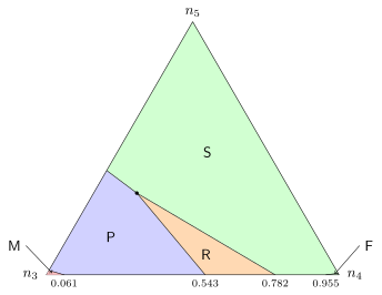
Figure 4: The row of Table 4 with the smallest bound for graphs of maximum degree at most \(5\), as a function of \((n_3,n_4,n_5)/(n_3+n_4+n_5)\) (Remark A.18; computed in floating point). A corner stands for the graphs all of whose vertices of degree at least \(3\) have that degree; the labels on the bottom edge give the proportion of degree-\(4\) vertices among those of degree \(3\) or \(4\). The region of \(\mathsf{F}\) is too thin to be visible.

A.4.2 Comparison with previous bounds, and refinements

This subsection compares the coefficients \(a_d\) of Theorem 1.3 with the previous ones (Remark A.19) and records refinements that follow from the same argument (Remark A.20).

Remark A.19 (comparison with previous coefficients).  The previous per-degree coefficients are those of Fomin, Gaspers, Saurabh and Stepanov (Fomin et al. 2009 Lemma 1) for \(d\le6\), namely \(\frac16,\frac13,\frac{13}{30},\frac{23}{45}\) at degrees \(3\) to \(6\), and the sequence \(g_{1/6}(d)\) of Edwards and McDermid (Edwards and McDermid 2015 Corollary 5.2) (recalled in Lemma 9.16), which agrees with them for \(d\le6\) and continues with \(g_{1/6}(7)=\frac{359}{630}\), \(g_{1/6}(8)=\frac{1553}{2520}\), \(g_{1/6}(9)=\frac{14827}{22680}\), \(g_{1/6}(10)=\frac{155273}{226800}\). Edwards and McDermid show \(g_{1/6}(d)=1-\frac{7/2}{d+1}+O(d^{-3})\) (Edwards and McDermid 2015, sec. 3.1.2). The previous bound in terms of edges is \(\frac{13}{75}m+o(m)\): for treewidth by Scott and Sorkin (Scott and Sorkin 2007 Corollary 21), and for pathwidth by Kneis, Mölle, Richter and Rossmanith (Kneis et al. 2009); it also follows from the bound of Edwards and McDermid, since \(\max_d2g_{1/6}(d)/d=\frac{13}{75}\), attained at \(d=5\). Table 7 compares these values with the bootstrap \(\sigma\) of \(\mathsf{S}\) and the coefficients \(a_d\) of Theorem 1.3.

Table 7: Per-degree coefficients, rounded to five decimals: the previous \(g_{1/6}(d)\) of (Edwards and McDermid 2015), which for \(d\le6\) are those of (Fomin et al. 2009) (where every degree \(d\ge7\) has coefficient \(1\)), the bootstrap \(\sigma_d\) of \(\mathsf{S}\), and the coefficients \(a_d\) of Theorem 1.3. The last row gives, for each sequence \(x\), the coefficient \(\max_d2x_d/d\) of \(m\) (their ratio in the last column).

\(d\)	\(g_{1/6}(d)\)	\(\sigma_d\)	\(a_d\)	\(a_d/g_{1/6}(d)\)
\(3\)	\(0.16667\)	\(0.15625\)	\(0.15625\)	\(0.938\)
\(4\)	\(0.33333\)	\(0.25000\)	\(0.25000\)	\(0.750\)
\(5\)	\(0.43333\)	\(0.34375\)	\(0.34375\)	\(0.793\)
\(6\)	\(0.51111\)	\(0.43750\)	\(0.43750\)	\(0.856\)
\(7\)	\(0.56984\)	\(0.50446\)	\(0.50446\)	\(0.885\)
\(8\)	\(0.61627\)	\(0.55804\)	\(0.55952\)	\(0.908\)
\(9\)	\(0.65375\)	\(0.60119\)	\(0.60357\)	\(0.923\)
\(10\)	\(0.68463\)	\(0.63676\)	\(0.63961\)	\(0.934\)
\(d\ge11\)	\(1-\frac{7/2}{d+1}+O(d^{-3})\)	\(1-\frac{129/32}{d+1}+O(d^{-3})\)	\(1-\frac{4}{d+1}\)	\(\to1\)
per edge	\(\frac{13}{75}\approx0.17333\)	\(\frac{7}{48}\approx0.14583\)	\(\frac{7}{48}\)	\(0.841\)

By Lemma 9.16, the coefficients of Theorem 1.3 are below \(g_{1/6}(d)\) at every degree \(d\ge3\), and the previous sequence never reaches the coefficient \(1-\frac4{d+1}\) that Theorem 1.3 has from degree \(11\) on.

The relative improvement over \(g_{1/6}\) (one minus the last column of Table 7) is largest at degree \(4\) and shrinks for large degrees. The deficit \(1-a_d\) is \(\frac{111/28}{d+1}\) for \(7\le d\le10\) and \(\frac{4}{d+1}\) for \(d\ge11\), instead of the deficit \(\frac{7/2}{d+1}+O(d^{-3})\) of \(g_{1/6}\). The bootstrap \(\sigma\) itself has deficit \(\frac{w_d}{d+1}\) with \(\frac{111}{28}\le w_d<\frac{129}{32}\) for \(d\ge7\) and \(w_d\to\frac{129}{32}\) by Proposition 9.13, so the ratio of the deficit of \(\sigma\) to that of \(g_{1/6}\) tends to \(\frac{129/32}{7/2}=\frac{129}{112}\approx1.152\). At degree \(3\) the coefficient \(\frac5{32}\) of Theorem 1.3 is above the cubic constant \(c_{3}\approx0.13982\) of Theorem 8.1; graphs in which vertices of degree \(3\) dominate get smaller bounds from the refinements of Remark A.20.

Remark A.20 (refinements).  The following bounds follow from Theorem 7.2 and Lemmas 9.3 and 9.7, each with a remainder \(o(n)\). Part (a) is the computation behind rows \(\mathsf{P}\) and \(\mathsf{R}\) of Corollary 9.5.

(a) The bootstraps of \(\mathsf{P}\) and \(\mathsf{R}\). Apply Lemma 9.3 with \(k=5\) to the triples \(\mathsf{P}=(F_3,0.2575,0.3667)\) and \(\mathsf{R}=(0.1455,0.2530,0.3600)\) of Theorem 7.2. Both triples are nondecreasing. Their increments are \((h_3,h_4,h_5)\approx(0.14016,\,0.11734,\,0.10920)\) for \(\mathsf{P}\) (using \(F_3<0.1401583\)) and \((0.1455,\,0.1075,\,0.1070)\) for \(\mathsf{R}\), so \(H_5=h_5\) equals \(0.1092\) and \(0.1070\), and \(b_5+H_5\le1\). At \(d=6\), \(\theta_6=(1-b_5-H_5)/6\) equals \(0.08735\) for \(\mathsf{P}\) and \(0.08883\ldots\) for \(\mathsf{R}\); in both cases \(\theta_6\le H_5\le3\theta_6\). By Lemma 9.6(iv), \(h_6=H_6=\theta_6\), so \(b_6=b_5+\theta_6\), and Lemma 9.7 with \(j=6\) gives \(d\,b_d=(d-2)\,b_{d-1}+b_{d-2}+1\) for \(d\ge7\). Rounded up, the resulting sequences \(\sigma^{\mathsf{P}}\) and \(\sigma^{\mathsf{R}}\) are rows \(\mathsf{P}\) and \(\mathsf{R}\) of Table 4; in particular \(\sigma^{\mathsf{P}}_6=0.45405\) and \(\sigma^{\mathsf{R}}_6=0.44883\ldots\).

Every graph satisfies \(\mathop{\mathrm{pw}}(G)\le\sum_{d\ge3}\sigma^X_dn_d+o(n)\) for each \(X\in\{\mathsf{P},\mathsf{R},\mathsf{S}\}\), where \(\sigma^{\mathsf{S}}:=\sigma\), hence \(\mathop{\mathrm{pw}}(G)\le\min_X\sum_{d\ge3}\sigma^X_dn_d+o(n)\). The sequences from \(\mathsf{P}\) and \(\mathsf{R}\) improve on \(\sigma\) only at degree \(3\): for \(d\ge4\), \(\sigma_d<\sigma^{\mathsf{R}}_d\) and \(\sigma_d<\sigma^{\mathsf{P}}_d\). (For \(4\le d\le6\) this follows from \(\sigma_4=\frac14<0.2530\), \(\sigma_5=\frac{11}{32}<0.3600\) and \(\sigma_6=\frac7{16}<0.4488\). For \(d\ge7\) the differences satisfy the homogeneous recurrence \(d\,e_d=(d-2)\,e_{d-1}+e_{d-2}\), whose coefficients are positive, and they are positive at \(d=5,6\).) They do not improve Corollary 1.4 either, since \(\sigma^{\mathsf{P}}_6\) and \(\sigma^{\mathsf{R}}_6\) exceed \(\frac7{16}\), so \(\max_d2\sigma^X_d/d\ge\sigma^X_6/3>\frac7{48}\).

(b) Average degree. The increments of \(\sigma^{\mathsf{P}}\), \(\sigma^{\mathsf{R}}\) and \(\sigma\) are nonincreasing from \(d=3\) on: for \(d\le6\) by the increments computed in (a) and by \(\sigma_d=\frac{3d-4}{32}\) (Proposition 9.13), and for \(d\ge7\) because \(h_d=H_d\le H_{d-1}=h_{d-1}\) by Lemma 9.7. So for each \(X\) the linear interpolation \(\bar\sigma^X\colon[2,\infty)\to\mathbb{R}\) of the points \((d,\sigma^X_d)\), \(d\ge2\), where \(\sigma^X_2=0\), is concave. Recall the average degree \(\bar d=2m/n\) (Section 9.5). Let \(n_{\ge3}\) be the number of vertices of degree at least \(3\) and, if \(n_{\ge3}\ge1\), let \(\hat d:=\frac1{n_{\ge3}}\sum_{d\ge3}d\,n_d\) be their average degree. Jensen’s inequality for \(\bar\sigma^X\) bounds \(\sum_{d\ge3}\sigma^X_dn_d\) from above in two ways: by \(\bar\sigma^X(\bar d)\,n\), with the weights \(n_d/n\) for \(d\ge2\), if \(\delta(G)\ge2\); and by \(\bar\sigma^X(\hat d)\,n_{\ge3}\), with the weights \(n_d/n_{\ge3}\) for \(d\ge3\). With (a) this gives \[\mathop{\mathrm{pw}}(G)\le\min_X\bar\sigma^X(\bar d)\,n+o(n)\quad\text{if }\delta(G)\ge2, \qquad \mathop{\mathrm{pw}}(G)\le\min_X\bar\sigma^X(\hat d)\,n_{\ge3}+o(n)\quad\text{if }n_{\ge3}\ge1.\] The second bound needs no condition on the vertices of degree at most \(2\). The condition \(\delta(G)\ge2\) in the first cannot be dropped, since adding isolated vertices can lower \(\bar d\) to \(2\), where the bound is \(o(n)\), without changing the pathwidth.

The minimum in the first bound is attained by \(\mathsf{P}\) for \(2\le\bar d\le3.5428\), by \(\mathsf{R}\) for \(3.5428\le\bar d\le3.7818\), and by \(\mathsf{S}\) from \(3.7818\) on; the breakpoints are numerical. Indeed, on \([2,3]\) all three interpolations pass through \((2,0)\), and \(\sigma^{\mathsf{P}}_3\) is the smallest value at \(3\); on \([3,4]\) the crossings are those of the three chords; and from \(4\) on, \(\sigma_d\) is the smallest value at every integer, by (a). For example, the minimum is \(F_3<0.1402\) at \(\bar d=3\) and about \(0.1988\) at \(\bar d=3.5\), compared with \(\frac7{96}\bar d\), that is, \(0.21875\) and \(0.2552\ldots\), from Corollary 1.4.

A.5 Proof of the algorithmic theorem

This subsection proves Theorem 10.1, restated below, following the outline and the roadmap of Section 10.1, and then Corollary 10.2 and Theorem 10.3.

Theorem 10.1 (precise form of Theorem 1.5; restated). In each case listed above there are a nondecreasing function \(\rho\colon\mathbb{N}\to[0,\infty)\) with \(\rho(n)=o(n)\) and two algorithms that, given \(G\in\mathcal C\), output a path decomposition of \(G\) in interval form, of width at most \(\beta(G)+\rho(n)\), and in the general case also at most \(\frac7{48}m+\rho(2m)\):

(a)  a Las Vegas algorithm, in expected \(n^{1+o(1)}\) bit operations;

(b)  a deterministic algorithm, in \(n^{2+o(1)}\) bit operations.

In the bootstrap and general cases, each algorithm uses in addition \(O(n(n+m))\) operations on integers of \(O(\log n)\) bits.

Besides the Las Vegas and deterministic algorithms of the theorem, the case proofs also analyze the randomized algorithm, which takes one sample of the labels within a budget of random draws and outputs its layout without checking the counts. The Las Vegas algorithm draws samples in the same way, without the budget, and checks the counts of each sample until one passes. The analysis also gives the following statement, which Theorem 10.1 does not need.

Remark A.21 (a randomized algorithm).  In each case of Theorem 10.1, the randomized algorithm outputs, in \(n(\log n)^{O(1)}\) bit operations (in the bootstrap and general cases, with the \(O(n(n+m))\) further operations of the theorem), a path decomposition of width at most \(\beta(G)+\rho(n)\), and in the general case also at most \(\frac7{48}m+\rho(2m)\), except with probability \(\pi(n)\), or \(\pi(n_{\ge1})\) in the bootstrap and general cases, where \(\pi(k)\to0\) as \(k\to\infty\) and \(n_{\ge1}\) is the number of non-isolated vertices of \(G\). This follows from the case proofs below and Appendix A.5.10.

A.5.1 Model, parameters and exact local labels

This subsection fixes the parameters as functions of \(n\), recalls the labels of Definition 5.2 in the multiplicative form used by the algorithms, and shows how their coefficients are computed. The algorithms use these coefficients, rounded to rationals, together with the finite distribution of Appendix A.5.2 in place of the Gaussian variables.

Parameters.

For an integer \(n\ge3\) put \[t:=\lceil\log_2(n+2)\rceil,\qquad h:=\max\bigl\{1,\lfloor\tfrac18\log_2t\rfloor\bigr\},\qquad K:=h,\qquad \gamma:=t^{-2},\qquad M:=2t^3+1,\] and \[\xi:=12\,t^{-7/4},\qquad p_t:=12\,t^{-11/4},\qquad \omega_d:=2(d+1)\,\varphi(0)\,\xi+p_t\quad(d\ge0).\] Here \(h\) is the locality radius of the labels, \(1/K\) is the step of the grid of thresholds, \(\gamma\) is the step of the finite distribution and \(M\) its number of points, and \(\xi\), \(p_t\), \(\omega_d\) are the error terms of Lemma A.24 and Corollary A.25. The parameters are always computed from the order of the input graph (in the bootstrap and general cases from \(n_{\ge1}\)), also when they are used for a subgraph.

The threshold \(n_2\).

Put \(n_2:=2^{2^{40}}\). For \(n\ge n_2\) we have \(t\ge2^{40}\), so \(h=\lfloor\frac18\log_2t\rfloor\ge5\) and \[\begin{equation*} \tag{A.4} 4^h=2^{2h}\le2^{\frac14\log_2t}=t^{1/4}. \end{equation*}\] Moreover the following inequalities hold for all \(n\ge n_2\):

(N1)  \(\xi<1/K\);

(N2)  \(\xi\varphi(0)+p_t\le5\cdot10^{-5}\);

(N3)  \(8\mu\,t^{1/2}n^{-1/2}\le\frac12\) for \(\mu=12K+3\), and hence for every \(\mu\le12K+3\).

Indeed, \(K=h\le\log_2t\le t\), so \(\xi K\le12t^{-3/4}<1\), and \(\xi\varphi(0)+p_t\le24\,t^{-7/4}\le24\cdot2^{-70}\). For (N3), put \(L=\log_2n\ge2^{40}\); then \(t\le L+1\le2L\) and \(\mu\le12t+3\le13t\), so \(8\mu t^{1/2}\le104\,t^{3/2}\le104\,(2L)^{3/2}\le2^{L/2-1}=\frac12n^{1/2}\).

For \(n<n_2\) we shall put \(\rho(n):=n\) and \(\pi(n):=0\); then every width claim is trivial, because every path decomposition of a graph with \(n\) vertices has width at most \(n-1\). All probabilistic and quantitative estimates below therefore assume \(n\ge n_2\).

Weights and path products.

Each case fixes an integer weight \(q(x)\in\{2,3,4\}\) for every vertex \(x\) of the graph to be labeled:

• cubic case: \(q\equiv2\); padded case: \(q\equiv3\); padded case of degree \(5\), used only for the cut sweep of Theorem 10.3: \(q\equiv4\);

• mixed cases, applied to graphs with \(\delta\ge3\) and \(\Delta\le5\), and switched case, applied to graphs with \(\delta\ge3\) and \(\Delta\le4\): \(q(x)=d(x)-1\).

For vertices \(v,w\) let \(P(v,w)\) be the minimum of the products \(\prod_{i=0}^{k-1}q(x_i)\) over all \(v\)–\(w\) paths \(v=x_0,x_1,\dots,x_k=w\), with \(P(v,v)=1\). The support \(B(v)\) of \(v\) is the ball \(B_h(v)\) in the cubic and padded cases (of degree \(4\) and \(5\)), and \(\{w:P(v,w)\le2^h\}\) in the mixed and switched cases. Since \(q\ge2\), a path with \(k\) edges has product at least \(2^k\); hence every \(w\in B(v)\) satisfies \(\mathop{\mathrm{dist}}(v,w)\le h\), so \(B(v)\subseteq B_h(v)\) in all cases.

Ideal labels.

Let \((Z_w)_w\) be independent standard normal variables and put \[X_v:=\sum_{w\in B(v)}P(v,w)^{-1/2}Z_w,\qquad \sigma_v^2:=\mathop{\mathrm{Var}}X_v=\sum_{w\in B(v)}\frac1{P(v,w)}\ \ (\ge1),\qquad Y_v:=X_v/\sigma_v .\] These are the labels of Definition 5.2 with truncation radius \(h\).

• In the cubic case \(P(v,w)=2^{\mathop{\mathrm{dist}}(v,w)}\), so the coefficients are the geometric coefficients \(2^{-\mathop{\mathrm{dist}}(v,w)/2}\), truncated at distance \(h\).

• In the padded case \(P(v,w)=3^{\mathop{\mathrm{dist}}(v,w)}\), so the coefficients are \(3^{-\mathop{\mathrm{dist}}(v,w)/2}\), truncated at distance \(h\); in the padded case of degree \(5\), \(P(v,w)=4^{\mathop{\mathrm{dist}}(v,w)}\).

• In the mixed and switched cases, the arc length \(\ell(x\to y)=\frac12\ln(d(x)-1)=\frac12\ln q(x)\) gives the directed distance \(D(v,w)=\frac12\ln P(v,w)\), so \(e^{-D(v,w)}=P(v,w)^{-1/2}\), and \(P(v,w)\le2^h\) is the truncation \(D(v,w)\le R\) with \(R:=\frac h2\ln2\).

This is the path-product form of Remark 5.3. Thus the integer \(h\) plays the role of the radius parameter \(R\) of Section 5. The cubic and padded cases use the padded labels of Definition 5.2(a) (with \(p=3\) and \(p=4\), and \(p=5\) in the padded case of degree \(5\)) with \(R=h\), and the mixed cases use the mixed labels of Definition 5.2(b) with \(R=\frac h2\ln2\). In this subsection we write \(h\) throughout.

The next lemma restates the edge correlation bounds of Section 5 for these labels. For \(h\ge5\) put \(\varepsilon_h:=1/h\) in the cubic and padded cases and \(\varepsilon_h:=8/(h-4)\) in the mixed and switched cases, and for an edge \(uv\) put \(r_{uv}:=r_*=r_{33}\) in the cubic case, \(r_{uv}:=r_{44}\) in the padded case, \(r_{uv}:=r_{55}\) in the padded case of degree \(5\), and \(r_{uv}:=r_{d(u)d(v)}\) in the mixed and switched cases.

Lemma A.22 (edge correlations).  Let \(h\ge5\). Every edge \(uv\) satisfies \(\mathop{\mathrm{Corr}}(Y_u,Y_v)\ge r_{uv}(1-\varepsilon_h)\).

Proof. In the cubic and padded cases this is Lemma 5.4 with radius \(h\) (with \(p=3\), \(4\) and \(5\)). In the mixed and switched cases it is Lemma 5.5 with \(\Delta_0=5\) and radius \(R=\frac h2\ln2\): the arc lengths lie between \(\ell_{\min}=\frac12\ln2\) and \(\ell_{\max}=\frac12\ln4=\ln2\), and its error term (5.4) is \[\varepsilon_R=\frac{2\ell_{\max}^2}{\ell_{\min}(R-2\ell_{\max})} =\frac{2(\ln2)^2}{\frac12\ln2\cdot(\frac h2-2)\ln2}=\frac8{h-4},\] which is positive and finite for \(h>4\).  ∎

Ball sizes.

For a graph with \(\Delta\le5\), the first bound of (4.1) gives \(|B_k(v)|\le1+5\sum_{i=0}^{k-1}4^i\le2\cdot4^k\) for every \(k\ge0\). With (A.4), for \(n\ge n_2\), \[\begin{equation*} \tag{A.5} |B(v)|\le2t^{1/4},\qquad|B_{h+1}(v)|\le8t^{1/4},\qquad|B_{2h+2}(v)|\le32\,t^{1/2}. \end{equation*}\]

Computing the coefficients.

For each \(v\), a breadth-first search to depth \(h\) finds \(B_h(v)\). In the cubic and padded cases \(P(v,w)=q^{\mathop{\mathrm{dist}}(v,w)}\). In the mixed and switched cases we run Dijkstra’s algorithm from \(v\) inside \(B_h(v)\), with path products of integers in place of path sums (all factors are at least \(1\), so Dijkstra’s algorithm applies). This computes \(P(v,w)\) correctly for every \(w\) with \(P(v,w)\le2^h\): a minimizing path has product at most \(2^h\), hence at most \(h\) edges, so all its vertices lie in \(B_h(v)\). For the other vertices of \(B_h(v)\) the computed value is at least the true value and so also exceeds \(2^h\).

The algorithms use rational roundings of the coefficients and of the standard deviations. Put \[\tilde c_{vw}:=\frac{\lfloor t^3P(v,w)^{-1/2}\rfloor}{t^3}\quad(w\in B(v)), \qquad \tilde\sigma_v:=\frac{\lfloor t^3\sigma_v\rfloor}{t^3}.\] Both are computed with integer square roots, using \(\lfloor\sqrt{\lfloor x\rfloor}\rfloor=\lfloor\sqrt x\rfloor\) for \(x\ge0\): \(\lfloor t^3P^{-1/2}\rfloor=\lfloor\sqrt{\lfloor t^6/P\rfloor}\rfloor\) and \(\lfloor t^3\sigma_v\rfloor=\lfloor\sqrt{\lfloor t^6\sigma_v^2\rfloor}\rfloor\), where \(\sigma_v^2=\sum_{w\in B(v)}1/P(v,w)\) is an exact rational. Then \[\begin{equation*} \tag{A.6} 0\le\tilde c_{vw}\le1,\qquad|\tilde c_{vw}-P(v,w)^{-1/2}|\le t^{-3},\qquad \tilde\sigma_v\ge1,\qquad|\tilde\sigma_v-\sigma_v|\le t^{-3}, \end{equation*}\] because \(P\ge1\) and \(\sigma_v\ge1\). The numbers \(P(v,w)\le4^h\le t^{1/4}\) and the numerators of \(\tilde c_{vw},\tilde\sigma_v\) have \(O(\log t)\) bits. For \(n\ge n_2\) the work per vertex is \(t^{O(1)}\) bit operations by (A.5); for \(n<n_2\) it is bounded by a constant. In total, computing the coefficients takes \(n(\log n)^{O(1)}\) bit operations.

A.5.2 A finite distribution for the Gaussian variables

The algorithms replace each \(Z_w\) by a random variable with finitely many rational values and rational probabilities, so that labels can be sampled and compared, and conditional expectations computed, in exact arithmetic. This subsection defines that distribution, couples it with the standard normal distribution, and defines the discrete labels that the algorithms sort.

The distribution.

The finite distribution puts on each point of a grid of step \(\gamma\) in \([-t,t]\) a weight proportional to a rational approximation of the standard normal density. For \(|j|\le t^3\) put \(x_j:=j\gamma\), so that \(|x_j|\le t\); there are \(M=2t^3+1\) such points. Let \(g_j:=1/T_j\), where \(T_j=\sum_{k<4t^2}(x_j^2/2)^k/k!\) is the Taylor polynomial of \(e^{x_j^2/2}\) with \(4t^2\) terms. Since \(y:=x_j^2/2\le t^2/2\) and \(k!\ge(k/e)^k\), the omitted terms satisfy \[0\le e^y-T_j\le\sum_{k\ge4t^2}\Bigl(\frac{ey}{k}\Bigr)^k \le\sum_{k\ge4t^2}\Bigl(\frac e8\Bigr)^k\le2\cdot0.34^{4t^2},\] so \(T_j=e^y(1-\delta_j)\) with \(0\le\delta_j\le2\cdot0.34^{4t^2}\le\frac12\), and \(|g_j-e^{-y}|=e^{-y}\delta_j/(1-\delta_j)\le4\cdot0.34^{4t^2}\le t^{-8}\) for \(t\ge2\). Put \[A_j:=\lfloor t^8g_j\rfloor,\qquad A:=\sum_{|i|\le t^3}A_i,\] and let \(\zeta\) be the random variable with \(\mathbb{P}(\zeta=x_j)=A_j/A\). Since \(g_0=1\), we have \(A_0=t^8>0\). Every \(A_j\) is an integer in \([0,t^8]\) and \(A\le3t^{11}\), so the probabilities have \(O(\log t)\) bits. Computing \(T_j\) exactly takes \(t^{O(1)}\) bit operations (it is a sum of \(4t^2\) rationals whose numerators and denominators have \(O(t^2\log t)\) bits), so computing the whole distribution takes \(t^{O(1)}=(\log n)^{O(1)}\) bit operations.

Lemma A.23 (coupling).  Let \(t\ge5\). There is a coupling of \(\zeta\) with a standard normal variable \(Z\) such that \(\mathbb{P}(|Z-\zeta|>\gamma)\le t^{-3}\).

Proof. We round \(Z\) to the grid, show that the distribution of the rounding is within total variation distance \(t^{-3}/10\) of the distribution of \(\zeta\), and then glue a maximal coupling of the two distributions to \(Z\).

Let \(\hat Z\) be the rounding of \(Z\) to the grid: \(\hat Z=x_j\) if \(Z\in[x_j-\frac\gamma2,x_j+\frac\gamma2)\) for some \(|j|\le t^3\), and \(\hat Z=\star\) (an extra point) otherwise. Write \(\nu\) for the distribution of \(\hat Z\), so \(\nu(x_j)=p_j:=\mathbb{P}(Z\in[x_j-\frac\gamma2,x_j+\frac\gamma2))\), and \(p_{\mathrm{out}}:=\nu(\star)\le\mathbb{P}(|Z|\ge t)\le e^{-t^2/2}\).

Midpoint rule. Put \(\bar q_j:=\gamma\varphi(x_j)\). Since \(\varphi''(z)=(z^2-1)\varphi(z)\) satisfies \(\sup|\varphi''|=\varphi(0)<0.4\), the midpoint rule gives \(|p_j-\bar q_j|\le\frac{\gamma^3}{24}\cdot0.4=\frac{t^{-6}}{60}\). Summed over the \(M\le3t^3\) points this is at most \(t^{-3}/20\).

Rational weights. Put \(\tilde a_j:=\gamma A_j/(t^8\sqrt{2\pi})\). Since \(|A_j/t^8-g_j|\le t^{-8}\) and \(|g_j-e^{-x_j^2/2}|\le t^{-8}\), we have \(|A_j/t^8-e^{-x_j^2/2}|\le2t^{-8}\), so \(|\tilde a_j-\bar q_j|\le\gamma\cdot2t^{-8}/\sqrt{2\pi}\le t^{-10}\); summed over \(j\) this is at most \(3t^{-7}\).

Total variation. Hence \[\sum_j|\tilde a_j-p_j|+p_{\mathrm{out}}\le e_t:=\frac{t^{-3}}{20}+3t^{-7}+e^{-t^2/2} \le\frac{t^{-3}}{10}\qquad(t\ge5),\] because \(3t^{-7}\le t^{-3}/40\) and \(e^{-t^2/2}\le t^{-3}/40\) for \(t\ge5\). The distribution of \(\zeta\) is \((\tilde a_j/\sum_i\tilde a_i)_j\), since \(\tilde a_j\) is proportional to \(A_j\). Normalizing changes the \(\ell_1\) distance to \(\nu\) by at most \(|1-\sum_i\tilde a_i|=|\sum_i(\tilde a_i-p_i)-p_{\mathrm{out}}|\le e_t\). So the \(\ell_1\) distance between the distribution of \(\zeta\) and \(\nu\) (on the points \(x_j\) and \(\star\)) is at most \(2e_t\), and the total variation distance is at most \(e_t\le t^{-3}/10\).

Coupling. Take a maximal coupling \((\hat Z',\zeta)\) of \(\nu\) and the distribution of \(\zeta\), so \(\mathbb{P}(\hat Z'\ne\zeta)\le t^{-3}/10\), and glue it to \((Z,\hat Z)\) along \(\hat Z=\hat Z'\) (draw \(Z\) from its conditional distribution given \(\hat Z=\hat Z'\)). On the event \(\zeta=\hat Z\), the common value is a grid point \(x_j\), because \(\zeta\) never equals \(\star\), and then \(|Z-\zeta|\le\gamma/2\). Hence \(\mathbb{P}(|Z-\zeta|>\gamma)\le\mathbb{P}(\zeta\ne\hat Z)\le t^{-3}\).  ∎

Discrete labels.

Let \((\tilde Z_w)_w\) be independent copies of \(\zeta\) and \[\tilde X_v:=\sum_{w\in B(v)}\tilde c_{vw}\tilde Z_w,\qquad \tilde Y_v:=\tilde X_v/\tilde\sigma_v .\] Each \(\tilde Y_v\) is a rational of the form \(a/(b\,t^2)\) with integers \(a,b\) of \(O(\log t)\) bits, so two labels, or a label and a rational threshold with \(O(\log t)\) bits, are compared in \((\log t)^{O(1)}\) bit operations. The algorithms order the vertices by \((\tilde Y_v,v)\) lexicographically; ties between labels are broken by the vertex index. For a rational \(\tau\) write \[\tilde S_\tau:=\{v:\ \tilde Y_v<\tau\},\] a prefix of this order. Note the strict inequality.

Sampling.

To sample \(\zeta\), draw \(\lceil\log_2A\rceil\) random bits, forming an integer \(U\); if \(U\ge A\), draw again; otherwise return the \(x_j\) with \(\sum_{i<j}A_i\le U<\sum_{i\le j}A_i\), found by binary search in the prefix sums. A draw succeeds with probability \(A/2^{\lceil\log_2A\rceil}>\frac12\), so a sample needs fewer than two draws in expectation, each of \(O(\log t)\) bits and \(O(\log M)\) comparisons. To keep the running time of the randomized algorithms bounded in the worst case, they draw at most \(2N\lceil\log_2n\rceil\) times in total for \(N\) samples; if this budget is exhausted they output the trivial decomposition with one bag \(V(G)\). By Markov’s inequality the budget is exhausted with probability less than \(1/\lceil\log_2n\rceil\). The Las Vegas algorithms have no budget.

A.5.3 Perturbation

We couple the discrete labels with the ideal labels so that, in the closed neighborhood of any fixed vertex, all labels move by at most \(\xi\) except with probability at most \(p_t\) (Lemma A.24). As a consequence, the per-vertex probabilities that bound the counts transfer from the ideal to the discrete labels, up to a shift of the threshold by \(\xi\) and an additive error that tends to zero as \(n\to\infty\) (Corollary A.25). So the analysis of the algorithms can use bounds on the ideal labels, which Appendix A.5.4 derives from Part I.

Lemma A.24 (perturbation).  Let \(n\ge n_2\), and let \(H\) be a graph with \(\Delta(H)\le5\) whose labels are built with the parameters of \(n\). There is a coupling of \((\tilde Y_v)_v\) with the ideal labels \((Y_v)_v\) such that every vertex \(v\) satisfies \[\mathbb{P}\bigl(|\tilde Y_u-Y_u|>\xi\ \text{for some}\ u\in N[v]\bigr)\le p_t .\]

Proof. Couple each pair \((\tilde Z_w,Z_w)\) by Lemma A.23 (\(t\ge2^{40}\ge5\)), independently over \(w\). The labels in \(N[v]\) use at most \(|N[v]|\cdot2t^{1/4}\le12t^{1/4}\) variables by (A.5), so with probability at least \(1-12t^{1/4}t^{-3}=1-p_t\) all of them satisfy \(|\tilde Z_w-Z_w|\le\gamma=t^{-2}\). On this event, for \(u\in N[v]\), using (A.6), \(|\tilde Z_w|\le t\) and \(|B(u)|\le2t^{1/4}\), \[\begin{split} |\tilde X_u-X_u|&\le\sum_{w\in B(u)}\Bigl(|\tilde c_{uw}-P(u,w)^{-1/2}|\,|\tilde Z_w| +P(u,w)^{-1/2}|\tilde Z_w-Z_w|\Bigr)\\ &\le2t^{1/4}(t^{-2}+t^{-2})=4t^{-7/4}. \end{split}\] Also \(|\tilde X_u|\le2t^{1/4}\cdot t\), and \(|1/\tilde\sigma_u-1/\sigma_u|=|\sigma_u-\tilde\sigma_u|/(\sigma_u\tilde\sigma_u)\le t^{-3}\) since \(\sigma_u,\tilde\sigma_u\ge1\). Hence \[|\tilde Y_u-Y_u|\le\frac{|\tilde X_u-X_u|}{\sigma_u} +|\tilde X_u|\,\Bigl|\frac1{\tilde\sigma_u}-\frac1{\sigma_u}\Bigr| \le4t^{-7/4}+2t^{5/4}t^{-3}=6t^{-7/4}\le\xi.\]  ∎

The coupling transfers per-vertex probabilities from ideal to discrete labels. Recall that \(S_\tau=\{v:Y_v\le\tau\}\) for the ideal labels, and \(\tilde S_\tau=\{v:\tilde Y_v<\tau\}\) for the discrete ones.

Corollary A.25 (transfer).  In the setting of Lemma A.24, let \(v\) be a vertex of degree \(d\) and \(\tau\in\mathbb{R}\). Then:

(a)  \(\mathbb{P}(v\in\partial^{+}\tilde S_\tau)\le\mathbb{P}(v\in\partial^{+}S_{\tau-\xi})+\omega_d\);

(b)  \(\mathbb{P}(v\in\partial^{-}\tilde S_\tau)\le\mathbb{P}(v\in\partial^{-}S_{\tau+\xi})+\omega_d\);

(c)  for every family \(\mathcal A\) of subsets of \(N[v]\), \(\mathbb{P}(\{u\in N[v]:\tilde Y_u<0\}\in\mathcal A)\le \mathbb{P}(\{u\in N[v]:Y_u<0\}\in\mathcal A)+\omega_d\);

(d)  for \(\tau\le\tau'\): \(\mathbb{P}(\tau\le\tilde Y_v<\tau')\le(\tau'-\tau+2\xi)\varphi(0)+p_t\), and \(\mathbb{P}(\tilde Y_v<\tau)\le\Phi(\tau)+\xi\varphi(0)+p_t\), \(\mathbb{P}(\tilde Y_v\ge\tau)\le\Phi(-\tau)+\xi\varphi(0)+p_t\).

Proof. Let \(\mathcal E\) be the event that \(|\tilde Y_u-Y_u|\le\xi\) for all \(u\in N[v]\), and \(\mathcal W\) the event that no \(Y_u\) with \(u\in N[v]\) lies in \([\tau-\xi,\tau+\xi]\). Each \(Y_u\) is standard normal, so \(\mathbb{P}(\mathcal W^c)\le(d+1)\cdot2\xi\varphi(0)\), and \(\mathbb{P}(\mathcal E^c)\le p_t\) by Lemma A.24. Hence \(\mathbb{P}(\mathcal E^c\cup\mathcal W^c)\le\omega_d\), and it suffices to prove the inclusions (a)–(c) on \(\mathcal E\cap\mathcal W\).

(a) Let \(v\in\partial^{+}\tilde S_\tau\): \(\tilde Y_v\ge\tau\) and some neighbor \(u\) has \(\tilde Y_u<\tau\). Then \(Y_v\ge\tau-\xi\), so \(Y_v>\tau+\xi>\tau-\xi\) on \(\mathcal W\); and \(Y_u<\tau+\xi\), so \(Y_u<\tau-\xi\) on \(\mathcal W\). Thus \(v\in\partial^{+} S_{\tau-\xi}\).

(b) Let \(v\in\partial^{-}\tilde S_\tau\): \(\tilde Y_v<\tau\) and some neighbor \(x\) has \(\tilde Y_x\ge\tau\). Then \(Y_v<\tau+\xi\), and \(Y_x\ge\tau-\xi\), so \(Y_x>\tau+\xi\) on \(\mathcal W\). Thus \(v\in\partial^{-}S_{\tau+\xi}\).

(c) Take \(\tau=0\). On \(\mathcal E\cap\mathcal W\), every \(u\in N[v]\) has \(|Y_u|>\xi\ge|\tilde Y_u-Y_u|\), so \(\tilde Y_u<0\) if and only if \(Y_u<0\). Hence the two sets in (c) coincide on \(\mathcal E\cap\mathcal W\).

(d) uses only the event \(|\tilde Y_v-Y_v|\le\xi\), which fails with probability at most \(p_t\): on it, \(\tau\le\tilde Y_v<\tau'\) implies \(\tau-\xi\le Y_v<\tau'+\xi\), an event of probability at most \((\tau'-\tau+2\xi)\varphi(0)\); \(\tilde Y_v<\tau\) implies \(Y_v<\tau+\xi\); and \(\tilde Y_v\ge\tau\) implies \(Y_v\ge\tau-\xi\).  ∎

A.5.4 Uniform ideal means

This subsection bounds the expected frontier sizes of the ideal labels uniformly in the threshold (Lemma A.26). The counts of the layouts are taken at the thresholds of a grid whose step \(1/K\) tends to zero with \(n\), and Corollary A.25 shifts these thresholds by \(\xi\). We therefore need the bounds of Part I on expected frontier sizes for all thresholds in an interval at once, with an error that tends to zero as \(h\to\infty\). In the cubic, padded and mixed cases the bounds of Part I have this form. In the cubic and padded cases the per-vertex bounds hold for every threshold. In the mixed cases Lemma 7.7 holds for every threshold in \([-3,3]\), because the continuity of the center bound (Lemma 6.3) turns the factor \(1-\varepsilon_R\) in the correlation bounds into an additive error \(205\,\varepsilon_R\) per vertex. The lemma below restates these bounds for the ideal labels of radius \(h\).

In the lemma, \(r_h:=r_*(1-1/h)\), where \(r_*=r_{33}\) is the edge correlation bound of the cubic case, and \(\varepsilon_{\mathrm{mix}}(h):=205\,\varepsilon_h=1640/(h-4)\), where \(\varepsilon_h=8/(h-4)\) is the error term of Lemma A.22 in the mixed cases.

Lemma A.26 (uniform ideal means).  Let \(h\ge5\) and let \((Y_v)\) be the ideal labels of radius \(h\) of a graph \(H\) with \(N\) vertices.

(a)  Cubic case, \(\Delta(H)\le3\). Every vertex \(v\) satisfies \(\mathbb{P}(v\in\partial^{+}S_\tau)\le\kappa(r_h)\) for every \(\tau\ge0\), \(\mathbb{P}(v\in\partial^{-}S_\tau)\le\kappa(r_h)\) for every \(\tau\le0\), and \[\begin{align*} \mathbb{P}\bigl(Y_v<0,\ \exists u\in N(v):Y_u\ge0\bigr) +\mathbf{1}_{d(v)=3}\mathbb{P}\bigl(Y_v\ge0,\ Y_u<0\ \forall u\in N(v)\bigr)&\le\kappa(r_h),\\ \mathbb{P}\bigl(Y_v\ge0,\ \exists u\in N(v):Y_u<0\bigr) +\mathbf{1}_{d(v)=3}\mathbb{P}\bigl(Y_v<0,\ Y_u\ge0\ \forall u\in N(v)\bigr)&\le\kappa(r_h). \end{align*}\]

(b)  Padded case, \(\Delta(H)\le4\). For every \(\tau\in\mathbb{R}\), \(\mathbb{E}|\partial^{+}S_\tau|\le(F_4+178/h)\,N\).

(c)  Mixed cases, \(\delta(H)\ge3\) and \(\Delta(H)\le5\). For every \(\tau\in[-3,3]\), \(\mathbb{E}|\partial^{+}S_\tau|\le\beta(H)+\varepsilon_{\mathrm{mix}}(h)\,N\).

Proof. (a) By Lemma A.22, the labels of \(v\) and its \(d(v)\le3\) neighbors form a centered Gaussian vector with unit variances and incident correlations at least \(r_h\). For \(\tau\ge0\), \(\{v\in\partial^{+}S_\tau\}\subseteq\{Y_v\ge\tau,\ \exists u\in N(v):Y_u\le\tau\}\), whose probability is at most \(\kappa(r_h)\) by Proposition 8.8. For \(\tau\le0\), apply Proposition 8.8 to the labels \(-Y\), which have the same incident correlations, at the threshold \(-\tau\ge0\): the event \(v\in\partial^{-}S_\tau\) is contained in \(\{-Y_v\ge-\tau,\ \exists x\in N(v):-Y_x\le-\tau\}\). The first of the two displayed inequalities is Lemma 8.9, because its events differ from those of Lemma 8.9 only by events on which some label equals \(0\), which have probability zero. The second is Lemma 8.9 applied to \(-Y\), in the same way.

(b) By Lemma A.22, the labels of \(v\) and its \(d(v)\le4\) neighbors form a vector as in Corollary 6.8 with \(d=4\) and \(r=r_{44}(1-1/h)\). So \(\mathbb{P}(v\in\partial^{+}S_\tau)\le f_{4,r_{44}(1-1/h)}(\tau)\). For \(|\tau|\le3\) this is at most \(f_{4,r_{44}}(\tau)+205\,r_{44}/h\le F_4+178/h\) by (6.6), Lemma 6.3(b) with \(\bar r=r_{33}\) and Definition 6.7; for \(|\tau|>3\) it is at most \(4\Phi(-3)<F_4\) (Proposition 6.9). Sum over \(v\).

(c) If \(h\le12\), then \(\varepsilon_{\mathrm{mix}}(h)\ge205\) and the claim is trivial, since \(\mathbb{E}|\partial^{+}S_\tau|\le N\). Let \(h\ge13\), so that \(\varepsilon_h<1\). In the mixed cases the ideal labels are the mixed labels of Definition 5.2(b) with \(R=\frac h2\ln2\), and \(\varepsilon_R=\varepsilon_h\) for this \(R\) (proof of Lemma A.22). The triple of the case is one of \(\mathsf{P},\mathsf{R},\mathsf{S}\), and all degrees of \(H\) lie in \(\{3,4,5\}\). So Lemma 7.7 gives \(\mathbb{E}|\partial^{+}S_\tau|\le\beta(H)+205\,\varepsilon_hN=\beta(H)+\varepsilon_{\mathrm{mix}}(h)\,N\) for every \(\tau\in[-3,3]\).  ∎

A.5.5 Counts and derandomization

This subsection shows that the counts are close to their means with high probability, and that the method of conditional expectations finds discrete labels for which they are close to their means for certain. The randomized and Las Vegas algorithms use the first statement, and the deterministic algorithm uses the second.

Counts.

Let \(H\) be a graph with \(N\) vertices and \(\Delta(H)\le5\), labeled with the parameters of some \(n\ge\max\{N,n_2\}\). A count is a random variable \(X_c=\sum_{v\in V(H)}I_{c,v}\), where each \(I_{c,v}\in\{0,1\}\) is a function of \((\tilde Z_w)_{w\in B_{h+1}(v)}\) that can be evaluated from these values in \(t^{O(1)}\) bit operations. For example, \(\mathbf{1}\{v\in\partial^{+}\tilde S_\tau\}\) is such an indicator for every rational \(\tau\) with \(O(\log t)\) bits, because it depends on the labels in \(N[v]\), and \(\tilde Y_u\) depends on \(\tilde Z_w\) for \(w\in B(u)\subseteq B_h(u)\subseteq B_{h+1}(v)\).

Greedy fixing.

Let \(X_1,\dots,X_\mu\) be counts, \(m_c:=\mathbb{E}X_c\), and \[\Psi:=\sum_{c=1}^\mu(X_c-m_c)^2 .\] Greedy fixing is the following deterministic procedure: fix \(\tilde Z_w\) for \(w\in V(H)\) one at a time, each time choosing a value \(x_j\) with \(A_j>0\) that minimizes the conditional expectation of \(\Psi\) given the values fixed so far.

Lemma A.27 (concentration and derandomization).  In this setting the following hold.

(a)  \(\mathbb{E}\Psi=\sum_c\mathop{\mathrm{Var}}X_c\le8\mu Nt^{1/2}\).

(b)  For every \(\lambda>0\), the probability that \(X_c>m_c+\lambda\) for some \(c\) is at most \(8\mu Nt^{1/2}/\lambda^2\).

(c)  Greedy fixing ends with values of all \(\tilde Z_w\), each of positive probability, for which \(\Psi\le8\mu Nt^{1/2}\), and hence \(|X_c-m_c|\le\sqrt{8\mu N}\,t^{1/4}\) for every \(c\).

(d)  The means \(m_c\) can be computed exactly with \(\mu N\,n^{o(1)}\) bit operations, and greedy fixing uses \(\mu N^2n^{o(1)}\) bit operations.

Proof. (a) Apply Lemma 4.10 with \(a=1\) and \(A_v=B_{h+1}(v)\): two indicators \(I_{c,u}\) and \(I_{c,v}\) can be dependent only if \(B_{h+1}(u)\cap B_{h+1}(v)\ne\emptyset\), that is, if \(v\in B_{2h+2}(u)\). By (A.5) there are at most \(32t^{1/2}N\) such ordered pairs, so \(\mathop{\mathrm{Var}}X_c\le8Nt^{1/2}\), and \(\mathbb{E}\Psi\) is the sum of these variances.

(b) Chebyshev’s inequality and a union bound over the \(\mu\) counts.

(c) Let \(\mathcal F\) be the values fixed before the step that fixes \(\tilde Z_w\). Then \[\mathbb{E}[\Psi\mid\mathcal F]=\sum_j\frac{A_j}{A}\,\mathbb{E}[\Psi\mid\mathcal F,\ \tilde Z_w=x_j],\] an average over the values of positive probability, so the minimizing value chosen by greedy fixing does not increase the conditional expectation. Initially it is \(\mathbb{E}\Psi\le8\mu Nt^{1/2}\) by (a). At the end all variables are fixed and \(\Psi\) is a number at most \(8\mu Nt^{1/2}\); each of its terms \((X_c-m_c)^2\) is at most \(\Psi\).

(d) Given fixed values \(\mathcal F\), \[\mathbb{E}\bigl[(X_c-m_c)^2\bigm|\mathcal F\bigr] =\Bigl(\sum_v\mathbb{E}[I_{c,v}\mid\mathcal F]-m_c\Bigr)^2 +\sum_{u}\ \sum_{v\in B_{2h+2}(u)}\mathop{\mathrm{Cov}}(I_{c,u},I_{c,v}\mid\mathcal F),\] because the unfixed variables are independent, so the conditional covariance vanishes when \(B_{h+1}(u)\cap B_{h+1}(v)=\emptyset\). Each term involves at most \(|B_{h+1}(u)\cup B_{h+1}(v)|\le16t^{1/4}\) variables by (A.5), and is computed exactly by enumerating the at most \(M^{16t^{1/4}}\) assignments of the unfixed ones among them, with probabilities that are products of the rationals \(A_j/A\). Since \(M\le3t^3\) and \(t\le2\log_2n\), \[M^{16t^{1/4}}=\exp\bigl(O(t^{1/4}\log t)\bigr) =\exp\bigl(O((\log n)^{1/4}\log\log n)\bigr)=n^{o(1)}.\] All numbers involved are rationals whose denominators are powers of \(A\) with exponent \(O(t^{1/4})\), and whose numerators have \(n^{o(1)}\) bits; each indicator is evaluated in \(t^{O(1)}\) bit operations. So each term takes \(n^{o(1)}\) bit operations, and one evaluation of \(\mathbb{E}[\Psi\mid\mathcal F]\), with its \(O(\mu Nt^{1/2})\) terms, takes \(\mu N\,n^{o(1)}\). The means \(m_c\) are computed in the same way with nothing fixed. Greedy fixing makes \(N\) steps with at most \(M\) candidates each, which gives \(\mu N^2n^{o(1)}\) bit operations.  ∎

In all our layouts \(\mu=O(K)=O(\log\log n)\), so the bounds in (d) become \(N\,n^{o(1)}\) and \(N^2n^{o(1)}\) bit operations. Below we use only upper bounds of the form \(X_c\le m_c+\lambda\), in the following form.

The three algorithms.

Let \(n\ge n_2\), \(N\le n\) and \(\mu\le12K+3\), and put \(\theta_{\mathrm D}(n):=\sqrt{8\mu n}\,t^{1/4}\) and \(\theta_{\mathrm R}(n):=n^{3/4}\). By Lemma A.27(c), greedy fixing ends with every count at most its mean plus \(\theta_{\mathrm D}(n)\). By Lemma A.27(b) with \(\lambda=n^{3/4}\), one sample has every count at most its mean plus \(\theta_{\mathrm R}(n)\) except with probability at most \(8\mu t^{1/2}n^{-1/2}\), which is at most \(\frac12\) by (N3). So the randomized algorithm, with its sampling budget, fails with probability at most \(\pi(n):=8(12K+3)t^{1/2}n^{-1/2}+1/\lceil\log_2n\rceil\) (as \(\mu\le12K+3\)), and the Las Vegas algorithm, which resamples until every count is at most its mean plus \(n^{3/4}\), needs at most two samples in expectation. In the padded, mixed and cubic cases below, it therefore suffices to bound the width when every count is at most its mean plus \(\theta\in\{\theta_{\mathrm D}(n),\theta_{\mathrm R}(n)\}\).

A.5.6 Undoing reductions

In the switched, mixed, bootstrap and general cases the algorithm first applies the reduction operations of Definition 4.2, possibly interleaved with vertex deletions, and decomposes the final graph. The proof of Lemma 4.5 constructs from this a decomposition of the original graph. This subsection shows that the construction can be carried out in near-linear time (Lemma A.28). If the final graph is empty, its path decomposition has no bags and width \(-1\).

Lemma A.28 (undoing reductions).  Let \(F\), \(D\) and \(R\) be as in Lemma 4.5, where \(F\) has \(n\) vertices and \(m\) edges. Given \(F\), \(D\), \(V(R)\) and a path decomposition of \(R\) of width \(w\) with \(s\) bags, a path decomposition of \(F\) of width at most \(|D|+w+3\log_2n+1\) with at most \(s+n\) bags can be computed with \(O(m+s+n\log n)\) operations on integers of \(O(\log n)\) bits, where both decompositions are in interval form.

Lean proof: Alg.undoWidth, Alg.undoNoFallback (what is formalised)

The algorithm does not need the sequence of operations itself; the sequence only guarantees the structure of Lemma 4.5(b). We first record two standard facts, in the form in which the algorithm uses them. Reduction operations take a graph of treewidth at most \(2\) to the empty graph and yield a tree decomposition of width at most \(2\) (Claim A.29). Every tree decomposition of a graph with \(N'\) vertices has a bag whose removal leaves components of at most \(N'/2\) vertices, and such a bag can be found in time linear in the size of the decomposition (Claim A.30).

Elimination bags.

Suppose that reduction operations are applied to a graph \(Q\) until none applies, and that the final graph is empty. Let \(u_1,u_2,\dots\) be the vertices of \(Q\) in the order of their removal, let \(\Gamma_i\) be the set of neighbors of \(u_i\) in the current graph when \(u_i\) is removed, and put \(X_i:=\{u_i\}\cup\Gamma_i\). The parent of node \(i\) is the node \(j\) of smallest index with \(u_j\in\Gamma_i\) (then \(j>i\)), and node \(i\) is a root if \(\Gamma_i=\emptyset\). We call the sets \(X_i\), with this forest, the elimination bags of the sequence.

Claim A.29.  Let \(Q\) be a graph with \(\mathop{\mathrm{tw}}(Q)\le2\). Applying reduction operations to \(Q\) in any order until none applies ends with the empty graph, and the elimination bags, with the roots of their forest joined into a tree, form a tree decomposition of \(Q\) of width at most \(2\).

Proof. First, the process ends with the empty graph. Each operation produces a minor of the current graph, since (R3) contracts the edge \(vx\) and the others delete a vertex; so every current graph has treewidth at most \(2\). A nonempty graph of treewidth at most \(k\) has a vertex of degree at most \(k\): in a tree decomposition of width at most \(k\) in which no bag is contained in a neighboring bag (contract tree edges violating this), either there is one bag, or a leaf bag contains a vertex outside its neighbor’s bag, and all neighbors of that vertex lie in the leaf bag. By (RP3), every vertex of degree at most \(2\) admits an operation, so the process continues until the graph is empty.

Next, we show that the elimination bags form a tree decomposition. In every operation, \(\Gamma_i\) is a clique of the graph after the operation: it has at most one vertex, or it is \(\{x,y\}\) and \(xy\) is present in (R4) and added in (R3). Every edge of \(Q\) joins \(u_i\) to \(\Gamma_i\), where \(u_i\) is its end removed first, because edges disappear only with their ends; so it lies in \(X_i\). Let \(u_a\in \Gamma_i\) with \(a>i\), and let \(j\) be the parent of \(i\). If \(j\ne a\), then \(j<a\), and \(u_a,u_j\in \Gamma_i\) are adjacent after step \(i\); this edge survives until step \(j\), so \(u_a\in \Gamma_j\). Repeating, the nodes containing \(u_a\) include a path from \(i\) to \(a\) in the forest, so the nodes containing any vertex form a connected subtree. Joining the roots by arbitrary edges keeps this property.  ∎

Claim A.30.  Let \(Q\) be a graph with \(N'\ge1\) vertices and let \((\mathcal T,(X_\nu)_\nu)\) be a tree decomposition of \(Q\). One can find, in time linear in \(|V(\mathcal T)|+\sum_\nu|X_\nu|\), a node \(\nu\) such that every component of \(Q-X_\nu\) has at most \(N'/2\) vertices.

Proof. Root \(\mathcal T\), and assign each vertex \(x\) to the node \(\mathrm{top}(x)\) closest to the root among the nodes whose bags contain \(x\). For a node \(\nu\) let \(\omega(\nu)\) be the number of vertices assigned to the subtree \(\mathcal T_\nu\) rooted at \(\nu\). Both are computed by one traversal. For a child \(\nu'\) of \(\nu\), the vertices assigned to \(\mathcal T_{\nu'}\) are exactly the vertices that occur in \(\mathcal T_{\nu'}\) but not in \(X_\nu\): the nodes containing a vertex form a subtree, so a vertex occurring both in \(\mathcal T_{\nu'}\) and outside it occurs in \(X_\nu\). Similarly, the vertices outside \(X_\nu\) not assigned to \(\mathcal T_\nu\) occur only outside \(\mathcal T_\nu\). A component of \(Q-X_\nu\) is connected and avoids \(X_\nu\), so all its vertices occur in the same component of \(\mathcal T-\nu\); hence it has at most \(\omega(\nu')\) vertices for some child \(\nu'\), or at most \(N'-\omega(\nu)\) vertices.

To find \(\nu\), start at the root, and while the current node has a child \(\nu'\) with \(\omega(\nu')>N'/2\), move to that child. At the final node \(\nu\), all children have \(\omega(\nu')\le N'/2\), and \(N'-\omega(\nu)<N'/2\) (if \(\nu\) is not the root, we moved to \(\nu\) because \(\omega(\nu)>N'/2\); if \(\nu\) is the root, \(\omega(\nu)=N'\)).  ∎

Proof of Lemma A.28. For each component \(C\) of \((F-D)-V(R)\) put \(S_C:=N_{F-D}(C)\subseteq V(R)\). By Lemma 4.5(b), \(S_C\) is empty, a single vertex, or the two ends of an edge of \(R\), and \(\mathop{\mathrm{tw}}(F[C])\le2\). The algorithm decomposes each \(F[C]\) separately, with width \(O(\log n)\), inserts this decomposition, with that bag added to each of its bags, after a bag of the decomposition of \(R\) that contains \(S_C\) (at the end if \(S_C=\emptyset\)), and adds \(D\) to every bag. In detail, it has four steps.

(1)  Components. Compute the components \(C\) of \((F-D)-V(R)\) and their sets \(S_C\) by breadth-first search, in \(O(n+m)\) time.

(2)  Decomposing a component. Fix \(C\), with \(N_C=|C|\). Apply reduction operations to \(F[C]\) in any order, keeping the vertices of degree at most \(2\) in a queue and testing adjacency for (R3) and (R4) with a balanced search tree of edges. By Claim A.29 this ends with the empty graph, and its elimination bags form a tree decomposition of \(F[C]\) of width at most \(2\) with \(N_C\) nodes. A graph of treewidth at most \(2\) has fewer than \(2N_C\) edges, and every operation adds at most one edge, so this step takes \(O(N_C\log n)\) operations.

(3)  Balanced recursion. Given a connected graph \(Q=F[C']\), \(C'\subseteq C\), with a tree decomposition of width at most \(2\), find by Claim A.30 a bag \(X\) such that every component of \(Q-X\) has at most \(|C'|/2\) vertices. For each component \(C''\) of \(Q-X\), restrict the tree decomposition to \(C''\): intersect every bag with \(C''\) and keep the nodes whose bags meet \(C''\). These nodes form a subtree, because \(Q[C'']\) is connected and the nodes containing the two ends of an edge share a node, so this is a tree decomposition of \(Q[C'']\) of width at most \(2\). Recurse on each component, concatenate the resulting path decompositions, and add \(X\) to every bag (if \(Q-X\) is empty, output the single bag \(X\)). By induction on \(|C'|\), the result has width at most \(3\lfloor\log_2|C'|\rfloor\): if \(Q-X\) is empty, the width is \(|X|-1\), which is \(0\) if \(|C'|=1\) and at most \(2\) otherwise; if not, each \(C''\) has \(\lfloor\log_2|C''|\rfloor\le\lfloor\log_2|C'|\rfloor-1\) because \(|C''|\le|C'|/2\), and adding the at most three vertices of \(X\) to bags of width at most \(3(\lfloor\log_2|C'|\rfloor-1)\) gives the bound. It has at most \(|C'|\) bags, since the bags \(X\) are nonempty. At one level of the recursion the components are disjoint, and a bag of at most three vertices meets at most three of them, so the work per level is linear in \(N_C\); there are at most \(\lfloor\log_2N_C\rfloor+1\) levels. In interval form, the vertices of \(X\) receive the interval of the whole block produced by the call. This step takes \(O(N_C\log N_C)\) operations.

(4)  Insertion. Let \(W_1,\dots,W_s\) be the decomposition of \(R\). For each \(C\) with \(S_C\ne\emptyset\) choose the index \(i_C:=\max_{x\in S_C}\mathrm{first}(x)\); then \(S_C\subseteq W_{i_C}\), because \(S_C\) is a vertex, or the two ends of an edge of \(R\), whose intervals intersect. Immediately after \(W_{i_C}\) insert the bags \(W_{i_C}\cup P\) for the bags \(P\) of the decomposition of \(F[C]\) from step 3, the components with the same index one after another. Append the decompositions of the components with \(S_C=\emptyset\) at the end, and finally add \(D\) to every bag.

Correctness. The result is a path decomposition of \(F\). Every vertex lies in a bag and \(D\) in all bags, which covers the edges at \(D\). An edge of \(F-D\) inside \(V(R)\) is an edge of \(R\) by Lemma 4.5(b), so it lies in some \(W_i\). Any other edge of \(F-D\) joins a vertex of some \(C\) to a vertex of \(C\cup S_C\), so it lies in a bag \(W_{i_C}\cup P\) or \(P\). A vertex of \(C\) occurs only in bags added for \(C\), and there in consecutive bags, since step 3 gives a path decomposition of \(F[C]\). A vertex \(x\in V(R)\) occurs in a run of consecutive bags \(W_i\) and in the bags inserted after them, since a bag inserted after \(W_i\) contains \(x\) exactly when \(x\in W_i\). As step 3 gives width at most \(3\log_2n\), the width is at most \(|D|+w+3\log_2n+1\), with at most \(s+\sum_CN_C\le s+n\) bags. (If no bag results, which happens only when \(F-D\) is empty, output the single bag \(D\).)

Interval form and running time. Let \(\ell_i\) be the total number of bags inserted after \(W_i\), and \(\mathrm{new}(i):=i+\sum_{i'<i}\ell_{i'}\) the new index of \(W_i\). A vertex \(x\) of \(R\) with interval \([\mathrm{first}(x),\mathrm{last}(x)]\) gets \([\mathrm{new}(\mathrm{first}(x)),\mathrm{new}(\mathrm{last}(x))+\ell_{\mathrm{last}(x)}]\), because the bags inserted after \(W_i\) contain \(x\) exactly when \(x\in W_i\). A vertex of a component \(C\) gets its interval within the block of \(C\), shifted by the position of the block, and every vertex of \(D\) gets the interval of all bags. Computing the \(\ell_i\), the prefix sums and the intervals takes \(O(n+s)\) time. Summing the running times of the four steps, using \(\sum_CN_C\le n\), gives \(O(m+s+n\log n)\).  ∎

A.5.7 The plain sweep: padded and mixed cases

This subsection proves Theorem 10.1 in the padded and mixed cases. The layout is the one of Lemma 4.1 for the order of the discrete labels, and its width is controlled by frontier sizes on the grid \[\tau_j:=-3+\frac jK\qquad(0\le j\le6K),\] together with the numbers of labels in the windows between grid points and in the two tails. Lemma A.31 bounds the width by these counts, and Proposition A.32 bounds the width when every count is at most its mean plus some \(\theta\ge0\), using the bounds on the means from Appendices A.5.3 and A.5.4. The algorithms ensure this condition, with high probability or for certain, by Lemma A.27; the proof of Theorem 10.1 in these cases ends the subsection.

The layout.

Let \(H\) be a graph with \(N\) vertices and \(\Delta(H)\le5\), with \(\delta(H)\ge3\) in the mixed cases, labeled with the parameters of some \(n\ge N\). Let \(v_1,\dots,v_N\) be the vertices in increasing order of \((\tilde Y_v,v)\) and \(T_i:=\{v_1,\dots,v_i\}\). The plain-sweep layout consists of the bags \(W_i:=\{v_i\}\cup\partial^{+}T_i\), \(1\le i\le N\). By Lemma 4.1, applied to any injective labeling that induces this order, it is a path decomposition of \(H\) of width \(\max_i|\partial^{+}T_i|\). By the definition of the bags, \(v_j\in W_i\) if and only if \(i=j\), or \(i<j\) and \(v_j\) has a neighbor in \(T_i\). So \(v_j\) occupies the bags \(W_{f_j},\dots,W_j\), where \(f_j\) is the smallest index \(k\) with \(k=j\) or \(v_k\in N(v_j)\), and the interval form is computed in \(O(N)\) time from the order.

Counts.

The plain sweep uses the \(\mu=12K+3\) counts \[\begin{align*} X^{\mathrm{fr}}_j&:=|\partial^{+}\tilde S_{\tau_j}|=\bigl|\{v:\ \tilde Y_v\ge\tau_j,\ \exists u\in N(v):\tilde Y_u<\tau_j\}\bigr| &&(0\le j\le6K),\\ X^{\mathrm{win}}_j&:=\bigl|\{v:\ \tau_j\le\tilde Y_v<\tau_{j+1}\}\bigr|&&(0\le j<6K),\\ X^{\mathrm{lo}}&:=\bigl|\{v:\ \tilde Y_v<-3\}\bigr|,\qquad X^{\mathrm{hi}}:=\bigl|\{v:\ \tilde Y_v\ge3\}\bigr| . \end{align*}\] Each is a count in the sense of Appendix A.5.5.

The following analogue of Lemma 7.8 works directly with the discrete labels, whose sublevel sets \(\tilde S_\tau\) are defined by a strict inequality.

Lemma A.31 (grid).  Every \(i\) satisfies \(|\partial^{+}T_i|\le\max\bigl\{5X^{\mathrm{lo}},\ X^{\mathrm{hi}},\ \max_{0\le j<6K}(X^{\mathrm{fr}}_{j+1}+X^{\mathrm{win}}_j)\bigr\}\).

Proof. Let \(y:=\tilde Y_{v_i}\). Every vertex of \(T_i\) has discrete label at most \(y\), and every vertex outside \(T_i\) has discrete label at least \(y\). Let \(u\in\partial^{+}T_i\), with a neighbor \(z\in T_i\); so \(\tilde Y_u\ge y\ge\tilde Y_z\).

• If \(y<-3\), then \(z\) is counted by \(X^{\mathrm{lo}}\). Each such \(z\) is a neighbor of at most \(5\) vertices \(u\), so \(|\partial^{+}T_i|\le5X^{\mathrm{lo}}\).

• If \(y\ge3\), then \(u\) is counted by \(X^{\mathrm{hi}}\).

• Otherwise \(\tau_j\le y<\tau_{j+1}\) for some \(0\le j<6K\). If \(\tilde Y_u\ge\tau_{j+1}\), then \(u\in\partial^{+}\tilde S_{\tau_{j+1}}\), because \(\tilde Y_z\le y<\tau_{j+1}\); so \(u\) is counted by \(X^{\mathrm{fr}}_{j+1}\). Otherwise \(\tau_j\le y\le\tilde Y_u<\tau_{j+1}\), and \(u\) is counted by \(X^{\mathrm{win}}_j\).

 ∎

Let \(\varepsilon(h)\) be the error term of Lemma A.26: \(\varepsilon(h):=178/h\) in the padded case and \(\varepsilon(h):=\varepsilon_{\mathrm{mix}}(h)\) in the mixed cases. Put \[\rho_0(n):=\varepsilon(h)+14\,\xi\varphi(0)+2p_t+\frac{\varphi(0)}K .\]

Proposition A.32 (plain sweep).  Let \(n\ge n_2\) and \(\theta\ge0\). If every count of the plain sweep is at most its mean plus \(\theta\), then the plain-sweep layout of \(H\) has width at most \(\beta(H)+\rho_0(n)N+5\theta\).

Proof. Frontier counts. Let \(1\le j\le6K\). By Corollary A.25(a), \(\mathbb{E}X^{\mathrm{fr}}_j\le\mathbb{E}|\partial^{+}S_{\tau_j-\xi}|+\omega_5N\). Since \(\tau_j\in[-3+1/K,3]\) and \(\xi<1/K\) by (N1), the threshold \(\tau_j-\xi\) lies in \([-3,3]\), and Lemma A.26 gives \(\mathbb{E}X^{\mathrm{fr}}_j\le\beta(H)+(\varepsilon(h)+12\xi\varphi(0)+p_t)N\) (in the padded case \(\beta(H)=F_4N\)).

Windows. By Corollary A.25(d), \(\mathbb{E}X^{\mathrm{win}}_j\le(\varphi(0)/K+2\xi\varphi(0)+p_t)N\).

Hence \(X^{\mathrm{fr}}_{j+1}+X^{\mathrm{win}}_j\le\beta(H)+\rho_0(n)N+2\theta\) for every \(0\le j<6K\).

Tails. By Corollary A.25(d) and (N2), \(\mathbb{E}X^{\mathrm{lo}}\) and \(\mathbb{E}X^{\mathrm{hi}}\) are at most \((\Phi(-3)+\xi\varphi(0)+p_t)N\le0.0014\,N\). So \(5X^{\mathrm{lo}}\) and \(X^{\mathrm{hi}}\) are at most \(0.007N+5\theta\). In every case \(\beta(H)\ge0.14N\): in the padded case \(F_4>0.14\), and in the mixed cases every vertex has degree at least \(3\) and every coefficient is at least \(0.14\). So \(0.007N+5\theta\le\beta(H)+5\theta\).

By Lemma A.31, every \(|\partial^{+}T_i|\), and hence the width, is at most \(\beta(H)+\rho_0(n)N+5\theta\).  ∎

The algorithms.

Let \(G\) be a graph of the padded or a mixed case, with \(n\ge3\) vertices (graphs with \(n\le2\) are decomposed by one bag). The randomized, Las Vegas and deterministic algorithms consist of the following four steps and differ only in step 3.

(1)  In the padded case put \(H:=G\). In the mixed cases apply reduction operations to \(G\) until none applies and let \(H\) be the final graph; it is empty or has \(\delta(H)\ge3\) by (RP3), and \(\Delta(H)\le\Delta(G)\) by (RP1). If \(H\) is empty, go to step 4.

(2)  Compute the parameters from \(n\), the coefficients \(\tilde c_{vw}\) and \(\tilde\sigma_v\) of \(H\), and the finite distribution.

(3)  Randomized: sample all \(\tilde Z_w\), compute the labels, sort, and build the plain-sweep layout. Las Vegas: also compute the means \(m_c\) of the counts; if \(n\ge n_2\) and some count exceeds \(m_c+n^{3/4}\), sample again. Deterministic: fix the \(\tilde Z_w\) by greedy fixing (Lemma A.27(c)), then build the layout.

(4)  In the mixed cases apply Lemma A.28 to \(F=G\), the performed reductions (\(D=\emptyset\)), and the layout of \(H\) (no bags if \(H\) is empty).

Proof of Theorem 10.1 in the padded and mixed cases. Let \(n\ge n_2\) (for \(n<n_2\) the claims are trivial, as explained in Appendix A.5.1). Since operations remove vertices and do not increase degrees by (RP1), and the coefficients are nonnegative and nondecreasing in the degree with \(a_0=a_1=a_2=0\), we have \(\beta(H)\le\beta(G)\). Let \[\theta_{\mathrm D}(n):=\sqrt{8(12K+3)n}\,t^{1/4},\qquad \theta_{\mathrm R}(n):=n^{3/4},\] \[\rho(n):=\rho_0(n)\,n+5\max\{\theta_{\mathrm D}(n),\theta_{\mathrm R}(n)\}+3\log_2n+1\] for \(n\ge n_2\), and \(\rho(n):=n\) for \(n<n_2\); we replace \(\rho\) by its running maximum (4.2). Then \(\rho(n)=o(n)\): we have \(\rho_0(n)\to0\), because \(h\to\infty\), \(\varepsilon(h)\to0\), \(\xi,p_t\to0\) and \(K=h\); and \(\theta_{\mathrm D}(n)=O(\sqrt{n\log\log n}\,(\log n)^{1/4})\).

When every count is at most its mean plus \(\theta\in\{\theta_{\mathrm D}(n),\theta_{\mathrm R}(n)\}\), with \(\mu=12K+3\) in the paragraph “The three algorithms” of Appendix A.5.5, Proposition A.32 bounds the width of the layout of \(H\) by \(\beta(G)+\rho_0(n)n+5\theta\), and Lemma A.28 adds at most \(3\log_2n+1\); so the width is at most \(\beta(G)+\rho(n)\). That paragraph gives the three algorithms, with failure probability \(\pi(n)\to0\) for the randomized one.

The running times are derived in Appendix A.5.10.  ∎

A.5.8 The median-switched layout: cubic case

This subsection proves Theorem 10.1 in the cubic case. The layout is the median-switched layout of Lemma 8.4: inner frontiers below threshold zero, a connector at zero, and outer frontiers above zero. Two points need care. First, the layout must be built for the discrete order, which is a lexicographic order with ties broken by vertex index rather than an order of distinct real labels; an auxiliary injective labeling \(y\) handles this. Second, the connector order of Lemma 8.3 must be computed efficiently (Lemma A.33). The counts and their means then bound the width as in Appendix A.5.7.

Let \(G\) be a graph with \(\Delta(G)\le3\) and \(n\ge3\) vertices; vertices of degree \(0\), \(1\) and \(2\) are allowed and no reductions are applied. The three algorithms are those of Appendix A.5.7 with \(H:=G\) and without steps 1 and 4, and with the layout below in place of the plain-sweep layout and the counts below in place of its counts. The labels use the weight \(q\equiv2\), and the counts use the grid \[\tau_j:=-2+\frac jK\qquad(0\le j\le4K),\qquad\text{so that }\tau_{2K}=0 .\]

An injective labeling for the discrete order.

Let \(\Sigma\) be the finite set \(\{\tilde Y_v:v\in V(G)\}\cup\{0\}\cup\{\tau_j:0\le j\le4K\}\), let \(\vartheta>0\) be so small that \(\vartheta n\) is less than every positive difference of two elements of \(\Sigma\), and put \[y_v:=\tilde Y_v+\vartheta v .\] The algorithms never compute \(y\); it is used only in the analysis.

• \(y\) is injective and induces the order of \((\tilde Y_v,v)\). If \(\tilde Y_u<\tilde Y_v\), then \(\tilde Y_v-\tilde Y_u>\vartheta n>\vartheta(u-v)\), so \(y_u<y_v\); if \(\tilde Y_u=\tilde Y_v\) and \(u<v\), then \(y_u<y_v\).

• Sublevel sets at the grid. For every \(\tau\in\Sigma\), \[S_\tau=\{v:\ y_v\le\tau\}=\tilde S_\tau=\{v:\ \tilde Y_v<\tau\}.\] If \(\tilde Y_v<\tau\), then \(\tau-\tilde Y_v>\vartheta n\ge\vartheta v\), so \(y_v<\tau\); if \(\tilde Y_v\ge\tau\), then \(y_v>\tilde Y_v\ge\tau\), since \(v\ge1\).

Here and below, \(S_\tau\), \(\partial^{-}S_\tau\), \(\partial^{+}S_\tau\), \(U\), \(W\), \(D\), \(U'\), \(W'\), \(L_0\) and \(L_0'\) are as in Section 8.1, for the labeling \(y\). We write \(\tau\) for the threshold called \(t\) there, because \(t\) is a parameter of this section. By the second item, \[\begin{align*} U&=\partial^{-}S_0=\{u:\ \tilde Y_u<0,\ \exists x\in N(u):\tilde Y_x\ge0\},\\ W&=\partial^{+}S_0=\{x:\ \tilde Y_x\ge0,\ \exists u\in N(x):\tilde Y_u<0\}, \end{align*}\] and \(D\) is the set of vertices of degree \(3\) all of whose neighbors lie on the other side of \(0\), where the two sides are \(\{\tilde Y<0\}\) and \(\{\tilde Y\ge0\}\).

The connector in linear time.

The connector of Lemma 8.4 needs an order of \(W'\) satisfying (8.3). The proof of Lemma 8.3 is a recursion on closed parts; the following order is computed directly. As in Lemma 8.3, let \(Q\) be a finite set and \(P\) a finite set of items, each item \(p\) having a nonempty set \(e(p)\subseteq Q\) of at most two endpoints. Let \(Q_1,\dots,Q_r\) be the vertex sets of the connected components of the hypergraph on \(Q\) whose edges are the sets \(e(p)\), \(p\in P\), indexed so that their excesses \(\mathrm{ex}_l:=|Q_l|-|\{p\in P:e(p)\subseteq Q_l\}|\) are nondecreasing in \(l\). A greedy order of \(Q_l\) starts with any element of \(Q_l\) and, as long as some item has one endpoint among the elements chosen so far and one outside them, adds the latter. A component order of \(Q\) is a concatenation of greedy orders of \(Q_1,\dots,Q_r\), in this order.

Lemma A.33 (connector in linear time).  Every component order is an ordering of \(Q\) that satisfies (8.3), and a component order can be computed in \(O(|Q|+|P|)\) time.

Lean proof: Alg.connectorLemma10, Alg.connectorNoFallback (what is formalised)

Proof. Every endpoint set is nonempty, connected in the hypergraph, and hence contained in exactly one \(Q_l\); so \(\sum_l\mathrm{ex}_l=|Q|-|P|\). Fix \(l\) and let \(X\) be the set of chosen elements of \(Q_l\) at some point, with \(\emptyset\ne X\subsetneq Q_l\). Since \(Q_l\) is connected, some edge \(e(p)\) meets both \(X\) and \(Q_l\setminus X\); as \(|e(p)|\le2\), \(p\) has one endpoint in \(X\) and one outside. So the greedy order continues until it exhausts \(Q_l\), and each step after the first covers an item that was not covered before; in particular, a component order is an ordering of \(Q\). Let \(c_l(j')\) be the number of items with \(e(p)\) contained in the first \(j'\) chosen elements of \(Q_l\); then \(c_l(j')\ge j'-1\) for \(j'\ge1\), so \(j'-c_l(j')\le1\) for all \(0\le j'\le|Q_l|\). In particular \(\mathrm{ex}_l=|Q_l|-c_l(|Q_l|)\le1\).

Now let \(j=\sum_{l<i}|Q_l|+j'\) with \(0\le j'\le|Q_i|\). The first \(j\) elements cover all items of \(Q_1,\dots,Q_{i-1}\), and the items of \(Q_i\) counted by \(c_i(j')\); no other item, since each item lies in one component. Hence \[j-c(j)=\sum_{l<i}\mathrm{ex}_l+\bigl(j'-c_i(j')\bigr)\le\sum_{l<i}\mathrm{ex}_l+1 .\] If \(\sum_{l<i}\mathrm{ex}_l>0\), then \(\mathrm{ex}_l>0\) for some \(l<i\), so \(\mathrm{ex}_{l'}\ge\mathrm{ex}_l>0\) for all \(l'\ge l\) by the ordering, and \(\sum_{l<i}\mathrm{ex}_l\le\sum_l\mathrm{ex}_l=|Q|-|P|\). Otherwise the sum is at most \(0\). In both cases \(j-c(j)\le\max(0,|Q|-|P|)+1\).

The components are found by breadth-first search in \(O(|Q|+|P|)\) time; the greedy orders are breadth-first searches as well. The excesses are integers in \([-|P|,1]\), so counting sort orders the components in \(O(|Q|+|P|)\) time.  ∎

The layout.

Let \(v_1,\dots,v_n\) be the vertices in increasing order of \((\tilde Y_v,v)\), which is the increasing order of \(y\), and \(\ell:=|\tilde S_0|\). The algorithms build the bags of Lemma 8.5: the inner bags \(A_1,\dots,A_\ell\), the connector bags \(C_{-1},C_0,\dots,C_k\) with \(k=|W'|\), and the outer bags \(A_{\ell+1},\dots,A_n\). The connector bags use a component order of \(W'\), computed by Lemma A.33 with \(Q=W'\) and the items \(P=\{u\in U':N(u)\cap W'\ne\emptyset\}\), where \(e(u)=N(u)\cap W'\); each item has at most two endpoints by Lemma 8.5. By Lemmas A.33 and 8.5, under the hypotheses of Lemma 8.4 these bags form a path decomposition of width at most \(w\). The sets \(U\), \(W\), \(D\), \(U'\), \(W'\) and \(P\) are computed in \(O(n)\) time from the signs of the labels. By the definitions of the bags, those containing a vertex are determined by its index, the smallest and largest indices of its neighbors, its position in the connector order, and the largest position of an element of \(e(u)\). So the interval form is computed in \(O(n)\) time after sorting.

Counts.

The cubic case uses the \(\mu=8K+4\) counts \[\begin{align*} X^{\mathrm{in}}_j&:=|\partial^{-}\tilde S_{\tau_j}|=\bigl|\{u:\ \tilde Y_u<\tau_j,\ \exists x\in N(u):\tilde Y_x\ge\tau_j\}\bigr|&&(0\le j<2K),\\ X^{\mathrm{out}}_j&:=|\partial^{+}\tilde S_{\tau_j}|&&(2K<j\le4K),\\ X^{\mathrm{win}}_j&:=\bigl|\{v:\ \tau_j\le\tilde Y_v<\tau_{j+1}\}\bigr|&&(0\le j<4K),\\ X^{\mathrm{lo}}&:=\bigl|\{v:\ \tilde Y_v<-2\}\bigr|,\qquad X^{\mathrm{hi}}:=\bigl|\{v:\ \tilde Y_v\ge2\}\bigr|, \end{align*}\] and \(L_0\), \(L_0'\). The last two are counts in the sense of Appendix A.5.5: \(L_0=\sum_v\mathbf{1}\{v\in U\cup(D\cap W)\}\), a disjoint union since \(U\cap W=\emptyset\), and each indicator depends only on the set \(\{u\in N[v]:\tilde Y_u<0\}\); similarly for \(L_0'=\sum_v\mathbf{1}\{v\in W\cup(D\cap U)\}\).

Means.

Let \(n\ge n_2\) and \(r_h=r_*(1-1/h)\), as in Appendix A.5.4. Then:

• for \(j<2K\) we have \(\tau_j+\xi\le-1/K+\xi<0\) by (N1), so Corollary A.25(b) and Lemma A.26(a) give \(\mathbb{E}X^{\mathrm{in}}_j\le(\kappa(r_h)+\omega_3)n\);

• for \(j>2K\) we have \(\tau_j-\xi\ge1/K-\xi>0\), so Corollary A.25(a) and Lemma A.26(a) give \(\mathbb{E}X^{\mathrm{out}}_j\le(\kappa(r_h)+\omega_3)n\);

• Corollary A.25(c) and the two switch inequalities of Lemma A.26(a) give \(\mathbb{E}L_0,\mathbb{E}L_0'\le(\kappa(r_h)+\omega_3)n\);

• Corollary A.25(d) gives \(\mathbb{E}X^{\mathrm{win}}_j\le(\varphi(0)/K+2\xi\varphi(0)+p_t)n\), and with (N2), \(\mathbb{E}X^{\mathrm{lo}},\mathbb{E}X^{\mathrm{hi}}\le(\Phi(-2)+\xi\varphi(0)+p_t)n<0.023\,n\).

Proof of Theorem 10.1 in the cubic case. Let \(n\ge n_2\) and suppose that every count is at most its mean plus \(\theta\). We check the hypotheses of Lemma 8.4 for \(y\) with \[w:=\bigl(\kappa(r_h)+\omega_3+\varphi(0)/K+2\xi\varphi(0)+p_t\bigr)n+2\theta+1 .\] Inner frontiers. Let \(\tau<0\). If \(\tau<-2\), then \(\partial^{-}S_\tau\subseteq S_\tau\subseteq S_{-2}=\tilde S_{-2}\), so \(|\partial^{-}S_\tau|\le X^{\mathrm{lo}}\le0.023n+\theta\). Otherwise \(\tau\in[\tau_j,\tau_{j+1})\) for some \(0\le j<2K\). Let \(u\in\partial^{-}S_\tau\), so \(y_u\le\tau<y_x\) for some neighbor \(x\). If \(y_u\le\tau_j\), then \(u\in\partial^{-}S_{\tau_j}\); otherwise \(\tau_j<y_u\le\tau_{j+1}\). Since \(S_{\tau_j}=\tilde S_{\tau_j}\) and \(S_{\tau_{j+1}}\setminus S_{\tau_j}=\{v:\tau_j\le\tilde Y_v<\tau_{j+1}\}\), this gives \(|\partial^{-}S_\tau|\le X^{\mathrm{in}}_j+X^{\mathrm{win}}_j\le w-1\).

Outer frontiers. Let \(\tau>0\). If \(\tau\ge2\), then \(\partial^{+}S_\tau\subseteq V(G)\setminus S_2\), so \(|\partial^{+}S_\tau|\le X^{\mathrm{hi}}\le0.023n+\theta\). Otherwise \(\tau\in[\tau_j,\tau_{j+1})\) for some \(2K\le j<4K\). Let \(x\in\partial^{+}S_\tau\), so \(y_x>\tau\ge y_u\) for some neighbor \(u\). If \(y_x>\tau_{j+1}\), then \(x\in\partial^{+}S_{\tau_{j+1}}\), and \(j+1>2K\); otherwise \(\tau_j\le\tau<y_x\le\tau_{j+1}\). So \(|\partial^{+}S_\tau|\le X^{\mathrm{out}}_{j+1}+X^{\mathrm{win}}_j\le w-1\).

Threshold zero. \(\max(L_0,L_0')+1\le(\kappa(r_h)+\omega_3)n+\theta+1\le w\).

Tails. \(0.023n+\theta\le w\), because \(\kappa(r_h)>c_{3}>0.023\); indeed \(\kappa\) is decreasing, since \(b(r)\) is increasing and \(\arccos\) is decreasing.

So Lemma 8.5 applies, and the decomposition built by the algorithms has width at most \(w\). Put \[\rho(n):=\bigl(\kappa(r_h)-c_{3}+\omega_3+\varphi(0)/K+2\xi\varphi(0)+p_t\bigr)n +2\max\{\theta_{\mathrm D}(n),\theta_{\mathrm R}(n)\}+1\] for \(n\ge n_2\), with \(\theta_{\mathrm D}(n)=\sqrt{8(8K+4)n}\,t^{1/4}\) and \(\theta_{\mathrm R}(n)=n^{3/4}\), and \(\rho(n):=n\) for \(n<n_2\); we replace \(\rho\) by its running maximum (4.2). Since \(\kappa\) is continuous and \(r_h\to r_*\), we have \(\kappa(r_h)\to c_{3}\), and \(\rho(n)=o(n)\).

The paragraph “The three algorithms” of Appendix A.5.5, with \(\mu=8K+4\), shows that the algorithms ensure this with \(\theta\in\{\theta_{\mathrm D}(n),\theta_{\mathrm R}(n)\}\), the randomized one except with probability \(\pi(n)\); then the width is at most \(c_{3}n+\rho(n)\).  ∎

A.5.9 The deletion process: bootstrap and general cases

This subsection proves Theorem 10.1 in the bootstrap cases and in the general case, by making the deletion process of Section 9 algorithmic. The bootstrap lemma is proved through the explicit bound (9.4), and the proof of that bound, through Proposition 9.10, is already a procedure: delete a vertex of maximum degree, reduce, and repeat until every component is basic. The induction of Edwards and McDermid (Edwards and McDermid 2015), which Proposition 9.10 generalizes, is of the same kind. The algorithm below makes the procedure explicit, with one simplification: it never tests whether a component is basic, which would require trying every vertex. Instead, it stops at a component of maximum degree at most \(k\) (defined below), which it decomposes by a sweep, and at a component that becomes empty when the chosen vertex is deleted and reduction operations are applied.

Throughout, \(X\) is one of the six sequences of Theorem 9.2, the seed, with base degree \(k\): \(k=3\) for \(\mathsf{C}\), \(k=4\) for \(\mathsf{M}\) and \(\mathsf{F}\), and \(k=5\) for \(\mathsf{P}\), \(\mathsf{R}\) and \(\mathsf{S}\). Let \((b_d)_{d\ge0}\) be the bootstrap of \(X\), with \(b_0=b_1=b_2=0\) and \((b_3,\dots,b_k)=X\); it satisfies the hypotheses of Lemma 9.6 (proof of Theorem 9.2). For \(X=\mathsf{S}\) it is denoted \(\sigma\) in Section 9.4; we keep the letter \(b\) of Section 9.1, because \(\sigma_v\) denotes standard deviations here. The sum \(\psi(G)=\sum_{d\ge3}b_dn_d(G)\), the potential \(\psi^-\) and the running minima \(H_d\) of the increments of \(b\) are as in Sections 9.1 and 9.3. The general case is the bootstrap case of \(\mathsf{S}\) with the coefficients rounded up: by Proposition 9.13, \(b_d\le a_d\) for every \(d\ge3\) when \(X=\mathsf{S}\), where \(a_d\) are the coefficients of Theorem 1.3.

Base layouts.

Each seed comes with a layout for graphs \(J\) with \(\delta(J)\ge3\) and \(\Delta(J)\le k\), labeled with the parameters of some \(n\ge\max\{|V(J)|,n_2\}\):

• \(\mathsf{C}\): the median-switched layout with the labels of the cubic case (\(q\equiv2\)), as in Appendix A.5.8;

• \(\mathsf{M}\): the median-switched layout with the labels of the switched case (\(q(x)=d(x)-1\)), as in Appendix A.6;

• \(\mathsf{F}\): the plain-sweep layout with the labels of the padded case (\(q\equiv3\));

• \(\mathsf{P}\), \(\mathsf{R}\), \(\mathsf{S}\): the plain-sweep layout with the labels of the mixed cases (\(q(x)=d(x)-1\)) and the triple \(X\).

For such a graph \(J\), \(\psi(J)=\sum_{d=3}^kb_dn_d(J)\), and this is the bound \(\beta(J)\) of the case whose labels are used; for \(\mathsf{C}\) and \(\mathsf{F}\) because every vertex of \(J\) has degree \(3\), respectively degree \(3\) or \(4\). Each base layout has at most \(12K+3\) counts in the sense of Appendix A.5.5, and if every count is at most its mean plus some \(\theta\ge0\), then the layout is a path decomposition of \(J\) of width at most \[\begin{equation*} \tag{A.7} \psi(J)+\rho_X(n)\,|V(J)|+5\theta+1, \end{equation*}\] where \(\rho_X(n)\) is the function \(\rho_0(n)\) of Appendix A.5.7 for the plain sweep (with the error term \(\varepsilon(h)\) of the case) and \(\rho_{\mathrm{med}}(n)\) of Appendix A.6 for the median-switched layout. This is Proposition A.32 for the plain sweep and Corollary A.39 for the median-switched layout.

The algorithm.

Let \(G_0\) be \(G\) without its isolated vertices, and \(n_{\ge1}:=|V(G_0)|\). If \(n_{\ge1}\le2\), output one bag \(V(G_0)\) and one bag for each isolated vertex. Otherwise compute all parameters from \(n_{\ge1}\), and an adjacency matrix of \(G_0\).

(1)  Apply reduction operations to \(G_0\) until none applies, recording the removed vertices; let \(R_0\) be the final graph.

(2)  Keep a list of components, initially those of \(R_0\), and a deleted set \(D:=\emptyset\). Repeat the following round while some component \(J\) in the list is not marked final:

• if \(\Delta(J)\le k\), mark \(J\) final (a sweep component);

• otherwise choose a vertex \(w\) of degree \(\Delta(J)\) that has a neighbor of smaller degree, if one exists, and any vertex of degree \(\Delta(J)\) otherwise. Apply reduction operations to \(J-w\) until none applies; let \(J^*\) be the final graph.

  • If \(J^*\) is empty, mark \(J\) final (a thin component). The deletion of \(w\) and these reductions are kept for step 3 only; they are not part of the global sequence. The reductions may have changed the shared adjacency matrix, so they are recorded in an undo log while they are applied and rolled back in time \(O(|V(J)|+|E(J)|)\), which restores \(J\).

  • Otherwise commit: add \(w\) to \(D\), record the deletion and the reductions as part of the global sequence, and replace \(J\) in the list by the components of \(J^*\).

(3)  Let \(R\) be the union of the final components. Decompose each sweep component \(J\) by the base layout of \(X\), with the parameters of \(n_{\ge1}\) (randomized, Las Vegas or deterministic, as below). Decompose each thin component \(J\) by Lemma A.28, applied to \(F=J\), the deleted set \(\{w\}\) and the empty final graph. Concatenate these decompositions into a decomposition of \(R\).

(4)  Apply Lemma A.28 to \(F=G_0\), the global sequence (deleted set \(D\), final graph \(R\)) and the decomposition of \(R\). Append one bag for each isolated vertex of \(G\).

By (RP2), reductions inside a component of the current graph are reductions of the whole current graph, so the global sequence is a sequence of reductions and deletions from \(G_0\) to \(R\), as Lemma A.28 requires. Every component in the list has minimum degree at least \(3\) by (RP3), since it is a component of the final graph of a maximal sequence of reductions. Every final component is basic in the sense of Definition 9.8: a sweep component has \(\Delta\le k\), and a thin component has the witness \(w\).

Lemma A.34 (the deletion process).  The algorithm makes at most \(n_{\ge1}\) commits and at most \(2n_{\ge1}\) rounds, and \(|D|+\psi^-(R)\le\psi(G)\).

Lean proof: Alg.deletionProcessBound (what is formalised)

Proof. Every commit deletes a vertex. Every other round marks a component final, and final components are disjoint, so there are at most \(n_{\ge1}\) of them.

Consider a commit at a component \(J\). Then \(J\) is connected, \(\delta(J)\ge3\), \(\Delta(J)\ge k+1\), the vertex \(w\) was chosen by the rule of Lemma 9.9, and \(J^*\) is the final graph of a maximal sequence of reductions applied to \(J-w\), and is nonempty. So Lemma 9.9 gives \(1+\psi^-(J^*)\le\psi^-(J)\). Hence the quantity \(|D|+\sum_J\psi^-(J)\), summed over the components in the list, does not increase at a commit, and it does not change when a component is marked final. At the start it is \(\psi^-(R_0)\) (by additivity), and at the end it is \(|D|+\psi^-(R)\). Finally \(\psi^-(R_0)\le\psi(R_0)\le\psi(G_0)=\psi(G)\), by (RP1), \(H\ge0\), and because isolated vertices have weight \(b_0=0\).  ∎

Proof of Theorem 10.1 in the bootstrap and general cases. Let \(n_{\ge1}\ge n_2\); otherwise the claims are trivial, because the output has width at most \(n_{\ge1}-1\) and we put \(\rho(N):=N\) and \(\pi(N):=0\) for \(N<n_2\). Put \[\begin{align*} \rho_{\mathrm{sw}}(N)&:=\rho_X(N)\,N+5\max\{\theta_{\mathrm D}(N),\theta_{\mathrm R}(N)\}+1,\\ \rho(N)&:=b_3+\rho_{\mathrm{sw}}(N)+6\log_2N+2\qquad(N\ge n_2), \end{align*}\] with \(\theta_{\mathrm D}(N)=\sqrt{8(12K+3)N}\,t^{1/4}\) and \(\theta_{\mathrm R}(N)=N^{3/4}\) (parameters of \(N\)); we replace \(\rho\) by its running maximum (4.2). Then \(\rho(N)=o(N)\), because \(\rho_X(N)\to0\).

We first bound the widths of the decompositions of the final components, of \(R\) and of \(G_0\), assuming that every count of every sweep component is at most its mean plus some \(\theta\le\max\{\theta_{\mathrm D}(n_{\ge1}),\theta_{\mathrm R}(n_{\ge1})\}\). Then we show that the three algorithms ensure this assumption, for certain or with the stated probability.

Sweep components. Let \(J\) be a sweep component with \(N_J\) vertices, and suppose that all its counts are at most their means plus \(\theta\le\max\{\theta_{\mathrm D}(n_{\ge1}),\theta_{\mathrm R}(n_{\ge1})\}\). By (A.7), applied with the parameters of \(n_{\ge1}\ge N_J\), its decomposition has width at most \(\psi(J)+\rho_X(n_{\ge1})N_J+5\theta+1\le\psi(J)+\rho_{\mathrm{sw}}(n_{\ge1})\). Since \(J\) is basic, \(\psi(J)\le\psi^-(J)+b_3\) by Lemma 9.11.

Thin components. By Lemma A.28 with deleted set \(\{w\}\) and \(R\) empty, the width is at most \(1+(-1)+3\log_2n_{\ge1}+1\).

The final graph. The width of the concatenation is the maximum over the components. Since \(\psi^-\) is nonnegative and additive, the decomposition of \(R\) has width at most \(\psi^-(R)+b_3+\rho_{\mathrm{sw}}(n_{\ge1})+3\log_2n_{\ge1}+1\).

Undoing. By Lemma A.28 and Lemma A.34, the decomposition of \(G_0\) has width at most \[|D|+\psi^-(R)+b_3+\rho_{\mathrm{sw}}(n_{\ge1})+6\log_2n_{\ge1}+2 \le\psi(G)+\rho(n_{\ge1})\le\sum_{d\ge3}b_dn_d(G)+\rho(n),\] using \(n_{\ge1}\le n\) and the monotonicity of \(\rho\). The bags of isolated vertices do not increase the width. This is the width bound of Theorem 10.1 in the bootstrap case of \(X\). In the general case, \(X=\mathsf{S}\) and \(b_d\le a_d\) give the first width bound, \(\sum_{d\ge3}a_dn_d(G)+\rho(n)\).

Edge bound (general case). Every vertex of \(G_0\) has degree at least \(1\), so \(n_{\ge1}\le2m\). By (9.9), \(a_d\le\frac7{48}\cdot\frac d2\) for every \(d\ge3\), and \(b_0=b_1=b_2=0\); so \(\psi(G)=\sum_db_dn_d(G)\le\frac7{48}\cdot\frac12\sum_vd(v)=\frac7{48}m\). Hence the same decomposition also has width at most \(\frac7{48}m+\rho(n_{\ge1})\le\frac7{48}m+\rho(2m)\).

Probability. The randomized algorithm samples the variables of different sweep components independently. We apply Lemma A.27(b) to each sweep component \(J\) with the global threshold \(\lambda=n_{\ge1}^{3/4}\): the probability that some count of \(J\) exceeds its mean plus \(n_{\ge1}^{3/4}\) is at most \(8\mu N_Jt^{1/2}n_{\ge1}^{-3/2}\), with \(\mu\le12K+3\). The sweep components are disjoint, so summing over them gives at most \(8(12K+3)t^{1/2}n_{\ge1}^{-1/2}\). With the sampling budget, which is \(2n_{\ge1}\lceil\log_2n_{\ge1}\rceil\) draws for the at most \(n_{\ge1}\) samples, the failure probability is at most \(\pi(n_{\ge1})\) with \(\pi(N):=8(12K+3)t^{1/2}N^{-1/2}+1/\lceil\log_2N\rceil\) (parameters of \(N\)). A union bound with each component’s own threshold \(N_J^{3/4}\) would not suffice, because there may be many components of moderate size.

Deterministic. Greedy fixing (Lemma A.27(c)) is run on each sweep component separately; the deviations are at most \(\sqrt{8\mu N_J}\,t^{1/4}\le\theta_{\mathrm D}(n_{\ge1})\).

Las Vegas. Steps 1, 2 and 4 are deterministic. In step 3, each sweep component is sampled, and resampled until all its counts are at most their means plus \(n_{\ge1}^{3/4}\). By Lemma A.27(b) and (N3), a sample of \(J\) is accepted with probability at least \(1-8\mu N_Jt^{1/2}n_{\ge1}^{-3/2}\ge\frac12\), so the expected number of samples per component is at most \(2\).  ∎

Remark A.35 (the rows and the sequences on all graphs).  The bootstrap of a seed \(X\) is entrywise at most the row \(X\) of Table 4, which rounds it up (for \(X\ne\mathsf{C}\); the bootstrap of \(\mathsf{C}\) is given in the caption), and at most the sequence \(X\) of Theorem 9.2, which agrees with it up to degree \(k\) and has coefficient \(1\) above \(k\) (Lemma 9.3). So the bootstrap cases compute, for every graph, decompositions of width at most the bound of each row of Corollary 9.5 and of each sequence of Theorem 9.2, plus the remainder \(\rho(n)\). No row is best for all graphs (Remark A.18); running the algorithm for each of the six seeds and keeping the narrowest decomposition realizes the minimum of the six bounds. For a graph of maximum degree at most \(k\), the bootstrap case of \(X\) never commits a deletion, and its bound \(\sum_{d=3}^kb_dn_d\) improves on the bound \(\beta(G)\) of the cubic and padded cases when \(G\) has vertices of degree at most \(2\).

A.5.10 Running times

The width claims of Theorem 10.1, and the probability claims of Remark A.21, are proved in Appendices A.5.7, A.5.8 and A.5.9 and Appendix A.6. This subsection bounds the running times of the steps of the algorithms, which completes the proof. Recall that \(t=O(\log n)\), that \(h,K=O(\log\log n)\), and that the number of counts is \(\mu=O(K)\).

Cubic, padded, switched and mixed cases.

Here \(m\le\frac52n\).

• Reductions (switched and mixed cases). Degrees never exceed \(5\), so each operation, including the adjacency test of (R3) and (R4), takes \(O(1)\) time with a queue of vertices of degree at most \(2\); in total \(O(n)\) operations on \(O(\log n)\)-bit integers, that is \(O(n\log n)\) bit operations.

• Coefficients and finite distribution. \(n(\log n)^{O(1)}\) and \((\log n)^{O(1)}\) bit operations (Appendices A.5.1 and A.5.2).

• Labels. Each \(\tilde Y_v\) is a sum of at most \(2t^{1/4}\) products of \(O(\log t)\)-bit rationals; in total \(n\,t^{O(1)}\) bit operations.

• Sampling (randomized). At most \(2n\lceil\log_2n\rceil\) draws of \(O(\log t)\) bits, each followed by a binary search over \(M\) prefix sums; in total \(n(\log n)^{O(1)}\) bit operations in the worst case.

• Sorting. \(O(n\log n)\) comparisons of labels, each in \((\log t)^{O(1)}\) bit operations.

• Layout. \(O(n)\) operations for the plain sweep; for the median-switched layout, \(O(n)\) operations by Lemma A.33 and the interval rules.

• Undoing. \(O(n\log n)\) operations by Lemma A.28, since the layout of \(H\) has \(s\le2N+2\le3n\) bags: \(N\) in the plain sweep, and \(N+|W'|+2\) in the median-switched layout.

So one sample (the randomized algorithm) uses \(n(\log n)^{O(1)}\) bit operations. The Las Vegas algorithm additionally computes the means in \(\mu n\,n^{o(1)}=n^{1+o(1)}\) bit operations (Lemma A.27(d)), checks the counts of each sample in \(n(\log n)^{O(1)}\) bit operations, and takes at most two samples in expectation; so its expected running time is \(n^{1+o(1)}\) (for \(n<n_2\) it accepts the first sample). The deterministic algorithm replaces sampling by greedy fixing (Lemma A.27(c)), which uses \(\mu n^2n^{o(1)}=n^{2+o(1)}\) bit operations.

Bootstrap and general cases.

Removing isolated vertices takes \(O(n)\) operations, and building the adjacency matrix of \(G_0\) takes \(O(n_{\ge1}^2)\).

• Steps 1 and 2. With adjacency lists that support deletion in \(O(1)\) time, the adjacency matrix for the tests and insertions of (R3) and (R4), and a queue of vertices of degree at most \(2\), each reduction takes \(O(1)\) operations. A component’s reductions after the deletion of \(w\) take \(O(|V(J)|+|E(J)|)\) operations, and so do the choice of \(w\) and the computation of the components of \(J^*\) by breadth-first search. By Lemma A.34 there are at most \(2n_{\ge1}\) rounds, so steps 1 and 2 take \(O(n_{\ge1}(n_{\ge1}+m))\) operations.

• Step 3. The sweep components are disjoint and have maximum degree at most \(5\), and each is decomposed by the base layout of the seed, so the bounds of the previous paragraph, summed over them, give \(n_{\ge1}(\log n_{\ge1})^{O(1)}\) bit operations (randomized), \(n_{\ge1}^{1+o(1)}\) in expectation (Las Vegas), and \(\sum_JN_J^2n_{\ge1}^{o(1)}\le n_{\ge1}^{2+o(1)}\) (deterministic). Each thin component takes \(O(|E(J)|+|V(J)|\log n_{\ge1})\) operations by Lemma A.28.

• Step 4. \(O(m+n_{\ge1}\log n_{\ge1})\) operations by Lemma A.28, since the decomposition of \(R\) has at most \(3n_{\ge1}\) bags: a component \(J\) contributes at most \(2|V(J)|+2\le3|V(J)|\) of them, as \(|V(J)|\ge4\).

In total, the bootstrap and general cases use \(O(n(n+m))\) operations on integers of \(O(\log n)\) bits, plus \(n(\log n)^{O(1)}\), expected \(n^{1+o(1)}\), or \(n^{2+o(1)}\) bit operations for one sample, the Las Vegas and the deterministic algorithm. This completes the proof of Theorem 10.1. \(\square\)

A.5.11 Orderings of small cutwidth

Notation.

We use the inner frontier \(\partial^{-}X=\{u\in X:N(u)\not\subseteq X\}\) of Section 4.2. Let \(e(X)\) be the number of edges with exactly one end in \(X\). For an ordering \((u_1,\dots,u_n)\) of \(V(G)\) with prefixes \(U_i=\{u_1,\dots,u_i\}\), the vertex separation of the ordering is \(\max_i|\partial^{-}U_i|\) and its cutwidth is \(\max_ie(U_i)\).

Lemma A.36 (cutwidth from vertex separation).  Let \(G\) be a graph with \(\Delta(G)\le3\) and \(n\ge1\) vertices, and let \((v_1,\dots,v_n)\) be an ordering of \(V(G)\) of vertex separation \(w\). Then an ordering of \(V(G)\) of cutwidth at most \(w+2\) can be computed in \(O(n)\) operations on integers of \(O(\log n)\) bits.

Proof. The relations \(s(G)\le\operatorname{vs}(G)+2\) ((Ellis, Sudborough, and Turner 1994 Lemma 2.2), half of their Theorem 2.1) and \(\operatorname{cw}(G)\le s(G)\) for maximum degree \(3\) ((Makedon and Sudborough 1989 Theorem 3.2), which gives their Corollary 3.3), where \(s\) is the search number, have constructive proofs; we check that they apply to the given ordering and run in linear time. Both papers work with connected multigraphs. Cutwidth and vertex separation of an ordering are maxima over the components (restrict the ordering to each component, then concatenate), so let \(G\) be connected.

Reduction. Let \(G'\) be obtained from \(G\) by suppressing, while possible, a vertex of degree \(2\) with two distinct neighbors (deleting it and joining its neighbors by an edge). This creates no loops, keeps all degrees, and takes \(O(n)\) operations. In \(G'\) every vertex of degree \(2\) is joined to a single vertex by two parallel edges, which is the form that the proof of (Makedon and Sudborough 1989 Theorem 3.2) brings the graph into (the reduction there, followed by subdividing every loop once). Restrict the given ordering to \(V(G')\). If \(u\in V(G')\) lies in a prefix and has a \(G'\)-neighbor outside it, then the path of \(G\) that the corresponding edge replaces leaves the prefix, and its last vertex in the prefix, counted from \(u\), has a \(G\)-neighbor outside it. This vertex is \(u\) or an inner vertex of a path at \(u\), so distinct such \(u\) give distinct vertices, and the restricted ordering of \(G'\) has vertex separation at most \(w\).

Searching. The procedure search1 in the proof of (Ellis, Sudborough, and Turner 1994 Lemma 2.2) takes the vertices of \(G'\) in this order, places a searcher on each, clears its edges to earlier vertices with one further searcher, and then removes the searchers from vertices with no uncleared edge. By the two invariants stated in that proof it never uses more than \(w+2\) searchers and never recontaminates an edge. This gives a search strategy \(S\) for \(G'\) with at most \(k=w+2\) searchers, without recontamination, with \(O(n)\) steps, and in which the step that clears each edge is known.

Ordering. The proof of (Makedon and Sudborough 1989 Theorem 3.2) orders the vertices of \(G'\) by the first step of \(S\) after which at least half of their incident edges are cleared, breaking ties by an explicit rule for vertices of degree \(2\), and shows that this ordering has cutwidth at most \(\lfloor\Delta(G')/2\rfloor(k-1)+1=k\). It is computed from the clearing steps by a bucket sort in \(O(n)\) operations.

Back to \(G\). Undo the suppressions in reverse order: an edge \(yz\) with \(y\ne z\) that replaced a vertex \(x\), with \(y\) before \(z\), becomes the path \(yxz\) with \(x\) placed directly after \(y\). The new cut between \(y\) and \(x\) is crossed by the same edges as the cut after \(y\) was, with \(yx\) in place of \(yz\); every other cut that \(yz\) crossed is now crossed by \(xz\) instead. So the cutwidth does not change, and the resulting ordering of \(V(G)\) has cutwidth at most \(w+2\).  ∎

Corollary 10.2 (computing orderings and bisections; restated). For graphs \(G\) with \(\Delta(G)\le3\), an ordering of \(V(G)\) of cutwidth at most \(c_{3}n+o(n)\), and a bisection of \(G\) with at most \(c_{3}n+o(n)\) edges between its two sides, can be computed in deterministic time \(n^{2+o(1)}\).

Proof. Theorem 10.1(b) computes a path decomposition \((W_1,\dots,W_r)\) of \(G\) of width at most \(c_{3}n+\rho(n)\), in interval form, in \(n^{2+o(1)}\) bit operations. Order the vertices by \(\mathrm{first}(v)\), breaking ties arbitrarily. Let \(L\) be a prefix of this ordering other than \(V(G)\), let \(u'\) be the first vertex after \(L\), and let \(g=\mathrm{first}(u')\), which is the least value of \(\mathrm{first}(y)\) over \(y\notin L\). If \(x\in L\) has a neighbor \(y\notin L\), then \(\mathrm{first}(x)\le g\le\mathrm{first}(y)\le j\) for a bag \(W_j\) that contains \(x\) and \(y\), so \(x\in W_g\). Hence \(\partial^{-}L\subseteq W_g\setminus\{u'\}\); since \(\partial^{-}V(G)=\emptyset\), the ordering has vertex separation at most \(c_{3}n+\rho(n)\). Lemma A.36 turns it into an ordering of cutwidth at most \(c_{3}n+\rho(n)+2\) in \(O(n\log n)\) bit operations. Splitting this ordering after its \(\lfloor n/2\rfloor\)-th vertex gives a bisection with at most as many edges between its two sides.  ∎

Theorem 10.3 (deterministic cut sweep; restated). Let \(p\in\{4,5\}\). For graphs \(G\) with \(\Delta(G)\le p\) and \(m\) edges, an ordering of \(V(G)\) of cutwidth at most \(\gamma_pm+o(n)\), and a bisection of \(G\) with at most that many edges between its two sides, can be computed in deterministic time \(n^{2+o(1)}\). For \(p=4\) the bound is \(\frac m6+o(n)\le\frac n3+o(n)\).

Proof. We use the padded labels of Appendix A.5.1: the padded case (\(q\equiv3\)) for \(p=4\) and the padded case of degree \(5\) (\(q\equiv4\)) for \(p=5\), with the parameters of \(n\); for \(n<n_2\) every ordering has cutwidth at most \(m\le\frac p2n\), which the remainder absorbs. Let \(n\ge n_2\), let \(v_1,\dots,v_n\) be the vertices in increasing order of \((\tilde Y_v,v)\), let \(T_i=\{v_1,\dots,v_i\}\), and let \(\tau_j=-3+j/K\) for \(0\le j\le6K\).

Counts. For \(0\le j<6K\) and \(1\le k\le p\) let \[\begin{align*} X^{\mathrm{cut}}_{j,k}&:=\bigl|\{v:\ \tilde Y_v<\tau_j,\ |\{u\in N(v):\tilde Y_u\ge\tau_j\}|\ge k\}\bigr|,\\ X^{\mathrm{win}}_{j,k}&:=\bigl|\{v:\ \tau_j\le\tilde Y_v<\tau_{j+1},\ d(v)\ge k\}\bigr|, \end{align*}\] and let \(X^{\mathrm{lo}}_k\) and \(X^{\mathrm{hi}}_k\) be the numbers of vertices \(v\) with \(d(v)\ge k\) and \(\tilde Y_v<-3\), respectively \(\tilde Y_v\ge3\). These \(\mu=p(12K+2)\) random variables are counts in the sense of Appendix A.5.5, since each indicator depends only on the labels in \(N[v]\). Summing over \(k\) turns the conditions \(c\ge k\) into the numbers \(c\), so \[C_j:=\sum_kX^{\mathrm{cut}}_{j,k}=e(\tilde S_{\tau_j}),\qquad D_j:=\sum_kX^{\mathrm{win}}_{j,k}=\sum_{v:\,\tau_j\le\tilde Y_v<\tau_{j+1}}d(v),\] and \(D^{\mathrm{lo}}:=\sum_kX^{\mathrm{lo}}_k\) and \(D^{\mathrm{hi}}:=\sum_kX^{\mathrm{hi}}_k\) are the degree sums over the two tails. (Each edge leaving \(\tilde S_{\tau_j}\) is counted once, at its end in \(\tilde S_{\tau_j}\).) We split the cut and the degree sums into counts because Lemma A.27 needs indicators.

Grid. Every prefix satisfies \[\begin{equation*} \tag{A.8} e(T_i)\le\max\Bigl\{D^{\mathrm{lo}},\ D^{\mathrm{hi}},\ \max_{0\le j<6K}(C_j+D_j)\Bigr\}. \end{equation*}\] Indeed, let \(y=\tilde Y_{v_i}\) and let \(zu\) be an edge with \(z\in T_i\) and \(u\notin T_i\), so \(\tilde Y_z\le y\le\tilde Y_u\). If \(y<-3\), we charge the edge to \(z\), which has \(\tilde Y_z<-3\) and receives at most \(d(z)\) edges; if \(y\ge3\), we charge it to \(u\), which has \(\tilde Y_u\ge3\). Otherwise \(\tau_j\le y<\tau_{j+1}\) for some \(j\). If \(\tilde Y_z<\tau_j\), the edge leaves \(\tilde S_{\tau_j}\), because \(\tilde Y_u\ge y\ge\tau_j\), and is counted by \(C_j\); otherwise \(\tau_j\le\tilde Y_z<\tau_{j+1}\), and we charge the edge to \(z\), counted by \(D_j\). This is the charging of the grid step in Section 3.4, for the discrete labels.

Means. Fix an edge \(uv\) and \(\tau\in\mathbb{R}\), and couple the discrete and ideal labels as in Lemma A.24. Let \(\mathcal E\) be the event that \(|\tilde Y_x-Y_x|\le\xi\) for \(x\in\{u,v\}\), which fails with probability at most \(p_t\) since \(\{u,v\}\subseteq N[u]\), and let \(\mathcal W\) be the event that neither \(Y_u\) nor \(Y_v\) lies in \([\tau-\xi,\tau+\xi]\), which fails with probability at most \(4\xi\varphi(0)\). If \(\tilde Y_u<\tau\le\tilde Y_v\), then on \(\mathcal E\cap\mathcal W\) we have \(Y_u<\tau+\xi\), hence \(Y_u<\tau-\xi\), and \(Y_v\ge\tau-\xi\), hence \(Y_v>\tau+\xi\): the edge crosses \(\tau\) for the ideal labels. The ideal labels have correlation at least \(r_{pp}(1-\frac1h)\) (Lemma A.22), so by Lemma 3.3(b) \[\mathbb{P}(uv\text{ leaves }\tilde S_\tau)\le\tfrac1\pi\arccos\bigl(r_{pp}(1-\tfrac1h)\bigr) +4\xi\varphi(0)+p_t=\gamma_p+o(1),\] uniformly in \(\tau\), because \(h\to\infty\) and \(\xi,p_t\to0\). Summing over the edges, \(\mathbb{E}C_j\le(\gamma_p+o(1))m\). By Corollary A.25(d) and (N2), a vertex lies in \([\tau_j,\tau_{j+1})\) with probability at most \(\varphi(0)/K+o(1)\), and below \(-3\) or at least \(3\) with probability at most \(0.0014\); as \(\sum_vd(v)=2m\), this gives \(\mathbb{E}D_j\le(2\varphi(0)/K+o(1))m=o(m)\) and \(\mathbb{E}D^{\mathrm{lo}},\mathbb{E}D^{\mathrm{hi}}\le0.0028\,m<\gamma_pm\).

Greedy fixing. By Lemma A.27(c), greedy fixing on these counts ends with values of the \(\tilde Z_w\) for which every count is within \(\theta=\sqrt{8\mu n}\,t^{1/4}=o(n)\) of its mean; so each of \(C_j\), \(D_j\), \(D^{\mathrm{lo}}\) and \(D^{\mathrm{hi}}\) is within \(p\theta\) of its mean. By (A.8), the sorted order has cutwidth at most \(\gamma_pm+o(n)\), and its first \(\lfloor n/2\rfloor\) vertices give the bisection. Since \(\mu=O(K)\), greedy fixing takes \(n^{2+o(1)}\) bit operations by Lemma A.27(d), and the other steps take \(n(\log n)^{O(1)}\) (Appendices A.5.1 and A.5.2). Finally \(\gamma_4=\frac16\) and \(m\le2n\) for \(p=4\).  ∎

A.6 Computing the median-switched decompositions

This subsection completes the proof of Theorem 10.1 where the median-switched layout of Section 8.2 is used outside Appendix A.5.8: in the switched case, which makes Theorem 8.2 algorithmic, and in the base layouts of the bootstrap cases \(\mathsf{C}\) and \(\mathsf{M}\) (Appendix A.5.9). The proof follows Appendix A.5.8, and two points are new. First, the layout must work for graphs whose labels are built with the parameters of an integer \(n\) larger than their number of vertices, as the sweep components of the deletion process require. Second, the existence proof of Theorem 8.2 bounds \(\mathbb{E}\hat L_0\) and \(\mathbb{E}\hat L_0'\) only in the limit of a large radius, so we make the error term explicit; together with the bounds at nonzero thresholds, this gives expected frontier sizes that are bounded uniformly in the threshold (Lemma A.37). We use the notation and the parameters of Section 10.

Two settings.

Let \(n\ge n_2\), and let \(H\) be a graph with \(N\le n\) vertices whose names are distinct positive integers. We consider two settings.

• Cubic setting: \(\Delta(H)\le3\), the labels are those of the cubic case (weight \(q\equiv2\)), and \(\beta(H):=c_{3}N\).

• Switched setting: \(\delta(H)\ge3\) and \(\Delta(H)\le4\), the labels are those of the switched case (weight \(q(x)=d(x)-1\), as in the mixed cases), and \(\beta(H):=c_{3}n_3(H)+0.2627\,n_4(H)\).

In both settings the labels are built with the parameters of \(n\). The construction of Appendices A.5.1 and A.5.2 and Lemmas A.22 and A.24 and Corollary A.25 apply, since they require only \(\Delta(H)\le5\), and \(\delta(H)\ge3\) for the weights \(q(x)=d(x)-1\). In the switched setting the edge correlation bounds are \(r_{uv}=r_{d(u)d(v)}\) with \(\varepsilon_h=8/(h-4)\). In both settings \(\beta(H)\ge c_{3}N\): in the cubic setting by definition, and in the switched setting because every vertex has degree \(3\) or \(4\) and both coefficients are at least \(c_{3}\).

Layout and counts.

Let \(\hat D\) be the set of vertices with at least three neighbors on the other side of zero, as in Appendix A.3.1, and \(\hat L_0=|U|+|\hat D\cap W|\) and \(\hat L_0'=|W|+|\hat D\cap U|\); in the cubic setting \(\hat D\) is the set \(D\) of Section 8.1, and \(\hat L_0=L_0\), \(\hat L_0'=L_0'\). The median-switched layout of \(H\) consists of the bags of Lemma 8.5, built as in Appendix A.5.8 from the order of \((\tilde Y_v,v)\), with \(\hat D\) in place of \(D\) and a component order of \(W'=W\setminus \hat D\) (Lemma A.33) for the items \(u\in U\setminus\hat D\) with \(e(u)=N(u)\cap W'\ne\emptyset\); each item has at most two endpoints by the definition of \(\hat D\). Its interval form is computed in \(O(N)\) time after sorting, as in Appendix A.5.8. The layout uses the grid \(\tau_j=-2+j/K\) (\(0\le j\le4K\)) and the \(\mu=8K+4\) counts of Appendix A.5.8: the inner counts \(X^{\mathrm{in}}_j\) (\(j<2K\)), the outer counts \(X^{\mathrm{out}}_j\) (\(j>2K\)), the windows \(X^{\mathrm{win}}_j\), the tails \(X^{\mathrm{lo}}\), \(X^{\mathrm{hi}}\), and \(\hat L_0\), \(\hat L_0'\) for the discrete labels. The last two are counts in the sense of Appendix A.5.5: \(\hat L_0=\sum_v\mathbf{1}\{v\in U\cup(\hat D\cap W)\}\), a disjoint union because \(U\cap W=\emptyset\), and the indicator depends only on the set \(\{u\in N[v]:\tilde Y_u<0\}\); similarly for \(\hat L_0'\).

Error terms.

Recall \(r_h=r_*(1-1/h)\) and \(\kappa\) from (8.1). For \(h\ge13\) we have \(\varepsilon_h=8/(h-4)\le\frac89\); put \[e_h:=205\,\varepsilon_h+\kappa\bigl(r_{33}(1-\varepsilon_h)\bigr)-c_{3},\qquad \varepsilon_{\mathrm{sw}}(h):=\max\bigl\{e_h,\ 12\,\varepsilon_h^{1/3}\bigr\}\qquad(h\ge13),\] and \(\varepsilon_{\mathrm{sw}}(h):=1\) for \(5\le h<13\). Let \(\varepsilon_{\mathrm{med}}(h)\) be \(\kappa(r_h)-c_{3}\) in the cubic setting and \(\varepsilon_{\mathrm{sw}}(h)\) in the switched setting. Since \(\kappa\) is continuous and \(\varepsilon_h\to0\), both tend to \(0\) as \(h\to\infty\). Put \[\rho_{\mathrm{med}}(n):=\varepsilon_{\mathrm{med}}(h)+\omega_4+\frac{\varphi(0)}K +2\xi\varphi(0)+p_t .\]

A.6.1 Uniform means in the switched setting

The proof of Theorem 8.2 bounds the expected frontiers at every nonzero threshold with the same error term \(e_R\) (Lemma A.14), so it is already uniform in the threshold. At threshold zero, Lemma A.11 makes the error term of Lemma A.12 explicit.

Lemma A.37 (uniform ideal means, switched setting).  Let \(h\ge5\), and let \((Y_v)\) be the ideal labels of radius \(h\) of a graph \(H\) with \(N\) vertices in the switched setting, and let \(S_\tau\), \(U\), \(W\), \(\hat D\), \(\hat L_0\) and \(\hat L_0'\) be defined for the labeling \(Y\). Then \[\begin{align*} \mathbb{E}|\partial^{+}S_\tau|&\le\beta(H)+\varepsilon_{\mathrm{sw}}(h)\,N\quad(\tau>0),\qquad \mathbb{E}|\partial^{-}S_\tau|\le\beta(H)+\varepsilon_{\mathrm{sw}}(h)\,N\quad(\tau<0),\\ \mathbb{E}\hat L_0&\le\beta(H)+\varepsilon_{\mathrm{sw}}(h)\,N,\qquad \mathbb{E}\hat L_0'\le\beta(H)+\varepsilon_{\mathrm{sw}}(h)\,N . \end{align*}\]

Proof. For \(h<13\) the claims are trivial, because each of the four quantities is at most \(N\) (\(\hat L_0\le|U\cup W|\) since \(U\cap W=\emptyset\), and similarly \(\hat L_0'\)). Let \(h\ge13\), so that \(\varepsilon_h<1\). By Lemma A.22, \((Y_v)\) is a centered Gaussian vector with unit variances and \(\mathop{\mathrm{Corr}}(Y_u,Y_v)\ge r_{d(u)d(v)}(1-\varepsilon_h)\) for every edge \(uv\). This is property (L1) of Section 7 with \(\varepsilon_h\) in place of \(\varepsilon_R\). Moreover \(-Y\) has the same distribution as \(Y\), because \(Y\) is a linear function of the independent standard normal variables \(Z_w\), and every \(Y_v\) has a continuous distribution, because \(Y_v\) has variance \(1\). The proofs of Lemmas A.14 and A.12 use the labels only through these properties: (L1), the sign symmetry and the continuity of the marginals.

Nonzero thresholds. Lemma A.14, with \(\varepsilon_h\) in place of \(\varepsilon_R\), gives \(\mathbb{E}|\partial^{+}S_\tau|\le\beta(H)+e_hN\) for \(\tau>0\) and \(\mathbb{E}|\partial^{-}S_\tau|\le\beta(H)+e_hN\) for \(\tau<0\), and \(e_h\le\varepsilon_{\mathrm{sw}}(h)\).

Threshold zero. Let \(v\) be a vertex of \(\{3,4\}\)-type \(T\), of degree \(d\le4\), with reference bounds \(r_T\) and transfer terms \(\lambda_T\) as in Definition 7.3. As in the proof of Lemma A.12, (A.2) and (L1) give \(\mathbb{P}(v\in U)+\mathbb{P}(v\in\hat D\cap W)\le M_d\bigl((1-\varepsilon_h)r_T\bigr)\), and Lemma A.11 with \(\gamma=\varepsilon_h\) gives \(M_d((1-\varepsilon_h)r_T)\le M_d(r_T)+3d\,\varepsilon_h^{1/3}\le\beta_T+12\,\varepsilon_h^{1/3}\), with \(\beta_T\) as in the table in that proof. By the second row of the table, with the transfer \(s=0.1529003-c_{3}\) of Appendix A.3.1, \[\mathbb{P}(v\in U)+\mathbb{P}(v\in\hat D\cap W)+\lambda_T(s,0,0)\le \begin{cases}c_{3}+12\,\varepsilon_h^{1/3}&\text{if }d=3,\\ 0.2627+12\,\varepsilon_h^{1/3}&\text{if }d=4.\end{cases}\] All degrees of \(H\) lie in \(\{3,4\}\), so Lemma 7.4, with the coefficients \(c_{3}\) and \(0.2627\) for the degrees \(3\) and \(4\) and with \(e=12\,\varepsilon_h^{1/3}\), gives \(\mathbb{E}\hat L_0\le\beta(H)+12\,\varepsilon_h^{1/3}N\). Up to null events, the events \(\{v\in W\}\) and \(\{v\in\hat D\cap U\}\) are the events \(\{v\in U\}\) and \(\{v\in\hat D\cap W\}\) for the labeling \(-Y\), which has the same distribution; so the same bound holds for \(\mathbb{E}\hat L_0'\).  ∎

In the cubic setting, Lemma A.26(a) gives the analogous per-vertex bounds, with \(\kappa(r_h)\) in place of \(c_{3}+\varepsilon_{\mathrm{sw}}(h)\).

A.6.2 The width of the median-switched layout

Proposition A.38 (median-switched sweep).  Let \(n\ge n_2\) and \(\theta\ge0\), and let \(H\) be a graph with \(N\le n\) vertices in the cubic or the switched setting. If every count of the median-switched layout is at most its mean plus \(\theta\), then this layout is a path decomposition of \(H\) of width at most \(\beta(H)+\rho_{\mathrm{med}}(n)\,N+2\theta+1\).

Proof. We first bound the means of the counts, then show that the layout is the path decomposition of Lemma 8.5 for an injective labeling that induces the order of \((\tilde Y_v,v)\), and finally check the hypotheses of that lemma.

Means. In the cubic setting the means are bounded in Appendix A.5.8, with \(N\) in place of \(n\) in the bounds and \(\omega_3\le\omega_4\); the argument does not use \(N=n\). In the switched setting we argue in the same way, with Lemma A.37 in place of Lemma A.26(a):

• for \(j<2K\), Corollary A.25(b) at the threshold \(\tau_j\), for which \(\tau_j+\xi<0\) by (N1), gives \(\mathbb{E}X^{\mathrm{in}}_j\le\mathbb{E}|\partial^{-}S_{\tau_j+\xi}|+\omega_4N\), since every degree is at most \(4\) and \(\omega_d\) is increasing in \(d\);

• for \(j>2K\), similarly Corollary A.25(a) gives \(\mathbb{E}X^{\mathrm{out}}_j\le\mathbb{E}|\partial^{+}S_{\tau_j-\xi}|+\omega_4N\) with \(\tau_j-\xi>0\);

• Corollary A.25(c), applied to the indicator of \(v\in U\cup(\hat D\cap W)\) as a function of the set of vertices of \(N[v]\) with negative label (for the ideal labels, \(Y_u<0\) and \(Y_u\le0\) differ by a null event), gives \(\mathbb{E}\hat L_0\le\mathbb{E}\hat L_0^{\mathrm{id}}+\omega_4N\), where \(\hat L_0^{\mathrm{id}}\) is \(\hat L_0\) for the ideal labels; similarly for \(\hat L_0'\);

• the windows and tails are bounded by Corollary A.25(d) and (N2): \(\mathbb{E}X^{\mathrm{win}}_j\le(\varphi(0)/K+2\xi\varphi(0)+p_t)N\) and \(\mathbb{E}X^{\mathrm{lo}},\mathbb{E}X^{\mathrm{hi}}<0.023N\).

With Lemma A.37 (switched setting) and Lemma A.26(a) (cubic setting), in both settings \[\mathbb{E}X^{\mathrm{in}}_j,\ \mathbb{E}X^{\mathrm{out}}_j,\ \mathbb{E}\hat L_0,\ \mathbb{E}\hat L_0' \le\beta(H)+(\varepsilon_{\mathrm{med}}(h)+\omega_4)\,N .\]

An injective labeling. Let \(\nu\) be the largest name of a vertex of \(H\), let \(\Sigma\) be the finite set \(\{\tilde Y_v:v\in V(H)\}\cup\{0\}\cup\{\tau_j:0\le j\le4K\}\), let \(\vartheta>0\) be so small that \(\vartheta\nu\) is less than every positive difference of two elements of \(\Sigma\), and put \(y_v:=\tilde Y_v+\vartheta v\). Exactly as in Appendix A.5.8, with \(\nu\) in place of \(n\), the labeling \(y\) is injective, induces the order of \((\tilde Y_v,v)\), and has sublevel sets \(S_\tau=\tilde S_\tau\) for every \(\tau\in\Sigma\). In particular \(U\), \(W\) and \(\hat D\) are the same for \(y\) as for the discrete labels. By Lemma 8.5 in the cubic setting, and by the same lemma with \(\hat D\) in place of \(D\) in the switched setting (which is established in the proof of Lemma A.9), the layout is a path decomposition of \(H\) of width at most \(w\) whenever \(w\) satisfies (i)–(iii) of Lemma 8.4 for \(y\), with \(\hat L_0\) and \(\hat L_0'\) in (iii); the component order satisfies (8.3) by Lemma A.33.

The hypotheses. Put \(w:=\beta(H)+\rho_{\mathrm{med}}(n)N+2\theta+1\), and assume that every count is at most its mean plus \(\theta\). For a threshold \(\tau<0\) with \(\tau\ge-2\), let \(\tau\in[\tau_j,\tau_{j+1})\) with \(j<2K\). The argument of Appendix A.5.8 gives \(|\partial^{-}S_\tau|\le X^{\mathrm{in}}_j+X^{\mathrm{win}}_j\), which is at most \[\beta(H)+(\varepsilon_{\mathrm{med}}(h)+\omega_4)N+\bigl(\varphi(0)/K+2\xi\varphi(0)+p_t\bigr)N +2\theta=w-1 .\] For \(0<\tau<2\), likewise \(|\partial^{+}S_\tau|\le X^{\mathrm{out}}_{j+1}+X^{\mathrm{win}}_j\le w-1\), where \(\tau\in[\tau_j,\tau_{j+1})\) with \(2K\le j<4K\). For \(\tau<-2\) and \(\tau\ge2\), the frontiers are bounded by the tails, which are at most \(0.023N+\theta\le c_{3}N+\theta\le\beta(H)+\theta\le w-1\). Finally, \(\max(\hat L_0,\hat L_0')+1\le\beta(H)+(\varepsilon_{\mathrm{med}}(h)+\omega_4)N +\theta+1\le w\). So (i)–(iii) hold, and the width is at most \(w\).  ∎

For \(H=G\) in the cubic setting, Proposition A.38 is the width bound proved in Appendix A.5.8, with \(\omega_4\) in place of \(\omega_3\).

A.6.3 The switched case

The algorithms.

Let \(G\) be a graph with \(\Delta(G)\le4\) and \(n\ge3\) vertices (graphs with \(n\le2\) are decomposed by one bag). The randomized, Las Vegas and deterministic algorithms are those of Appendix A.5.7, with the following changes. In step 1, reduction operations are applied to \(G\) until none applies; the final graph \(H\) is empty or has \(\delta(H)\ge3\) by (RP3), and \(\Delta(H)\le4\) by (RP1), so it is in the switched setting. In step 2 the coefficients of \(H\) use the weights \(q(x)=d_H(x)-1\). In step 3 the algorithms build the median-switched layout of \(H\) and use its \(8K+4\) counts. Step 4 applies Lemma A.28 as in the mixed cases.

Proof of Theorem 10.1 in the switched case. Let \(n\ge n_2\); for \(n<n_2\) the claims are trivial (Appendix A.5.1). The coefficients \((0,0,0,c_{3},0.2627)\) are nonnegative and nondecreasing in the degree, and reductions remove vertices and increase no degree by (RP1), so \(\beta(H)\le\beta(G)\). Put \[\rho(n):=\rho_{\mathrm{med}}(n)\,n+2\max\{\theta_{\mathrm D}(n),\theta_{\mathrm R}(n)\} +3\log_2n+2\qquad(n\ge n_2),\] with \(\theta_{\mathrm D}(n)=\sqrt{8(8K+4)n}\,t^{1/4}\) and \(\theta_{\mathrm R}(n)=n^{3/4}\), and \(\rho(n):=n\) for \(n<n_2\); we replace \(\rho\) by its running maximum (4.2). Then \(\rho(n)=o(n)\), because \(\rho_{\mathrm{med}}(n)\to0\). The three algorithms ensure that every count is at most its mean plus \(\theta\), exactly as in Appendices A.5.7 and A.5.8: deterministically with \(\theta=\theta_{\mathrm D}(n)\) by Lemma A.27(c); in the randomized algorithm with \(\theta=n^{3/4}\), except with probability at most \(\pi(n):=8(8K+4)t^{1/2}n^{-1/2}+1/\lceil\log_2n\rceil\); and in the Las Vegas algorithm with \(\theta=n^{3/4}\), which accepts a sample with probability at least \(\frac12\) by Lemma A.27(b) and (N3). In each case Proposition A.38, applied with \(N=|V(H)|\le n\), bounds the width of the layout of \(H\) by \(\beta(G)+\rho_{\mathrm{med}}(n)n+2\theta+1\), and Lemma A.28 adds at most \(3\log_2n+1\). So the width is at most \(\beta(G)+\rho(n)\). The running times are those of the cubic case (Appendix A.5.10): the reductions take \(O(n)\) operations, since degrees never exceed \(4\), and the coefficients are computed as in the mixed cases.  ∎

A.6.4 The sweep components of the bootstrap cases \(\mathsf{C}\) and \(\mathsf{M}\)

In the bootstrap case of a seed \(X\) (Appendix A.5.9), the deletion process stops at sweep components \(J\) with \(\delta(J)\ge3\) and \(\Delta(J)\le k\), where \(k=3\) for \(X=\mathsf{C}\) and \(k=4\) for \(X=\mathsf{M}\), and decomposes them with the parameters of the number \(n_{\ge1}\ge|V(J)|\) of non-isolated vertices of the input graph.

Corollary A.39 (base layouts for \(\mathsf{C}\) and \(\mathsf{M}\)).  Let \(X\in\{\mathsf{C},\mathsf{M}\}\) with base degree \(k\), let \(n\ge n_2\) and \(\theta\ge0\), and let \(J\) be a graph with \(\delta(J)\ge3\), \(\Delta(J)\le k\) and \(N_J\le n\) vertices, labeled in the cubic setting if \(X=\mathsf{C}\) and in the switched setting if \(X=\mathsf{M}\), with the parameters of \(n\). If every count of the median-switched layout of \(J\) is at most its mean plus \(\theta\), then the layout is a path decomposition of \(J\) of width at most \(\sum_{d=3}^kb_dn_d(J)+\rho_{\mathrm{med}}(n)N_J+2\theta+1\), where \((b_3,\dots,b_k)=X\).

Proof. For \(X=\mathsf{C}\) the graph \(J\) is \(3\)-regular, so \(\beta(J)=c_{3}N_J=c_{3}n_3(J)\). For \(X=\mathsf{M}\), \(\beta(J)=c_{3}n_3(J)+0.2627\,n_4(J)\). In both cases Proposition A.38 gives the claim.  ∎

A.7 Proofs for Part II

This subsection proves Lemma 11.2 (Appendix A.7.1), the statements on bucketing (Appendix A.7.2) and Theorem 14.1 (Appendix A.7.3). The analyses for Sections 12 and 13 are in Appendices C and D.

A.7.1 Pathwidth in terms of the vertices of degree three

Lemma 11.2 (pathwidth by the number of degree-\(3\) vertices; restated). There is a nondecreasing function \(\rho\colon\mathbb{N}\to\mathbb{R}\) with \(\rho(k)=o(k)\) such that every graph \(H\) with \(\Delta(H)\le3\) satisfies \[\mathop{\mathrm{pw}}(H)\le c_{3}\,n_3(H)+\rho\bigl(n_3(H)\bigr).\] A path decomposition of this width can be computed in polynomial time.

Proof. Let \(\rho_1\colon\mathbb{N}\to\mathbb{R}\) be the larger of the remainder of Theorem 8.1 and the remainder of the deterministic algorithm of Theorem 1.5 for that bound; replacing it by its running maximum (4.2), we take \(\rho_1\) nonnegative and nondecreasing. We prove the lemma with \[\rho(k):=\rho_1(k)+\log_2(2k+2)+6\qquad(k\in\mathbb{N}).\] Write \(n_3:=n_3(H)\). The proof has four steps: we remove the trees outside the \(2\)-core of \(H\), suppress the vertices of degree \(2\) of the core and decompose the simple graph underlying the resulting cubic multigraph by Theorem 8.1, and then put back first the suppressed paths and then the trees.

Step 1: the \(2\)-core. Repeatedly delete a vertex of degree at most \(1\) until none is left, and call the resulting graph \(H'\) (possibly empty). No degree increases, so \(n_3(H')\le n_3\). Every component \(T\) of \(H-V(H')\) is a tree with at most one edge to \(H'\). Otherwise \(T\) together with \(H'\) contains a cycle through a vertex of \(T\), or a path between two vertices of \(H'\) whose interior lies in \(T\); the first vertex of this cycle or path to be deleted had two neighbors at the time of its deletion, a contradiction.

Step 2: the core. Every vertex of \(H'\) has degree \(2\) or \(3\). Components of \(H'\) that are cycles have pathwidth at most \(2\). In every other component, every maximal path whose interior vertices have degree \(2\) joins two vertices of degree \(3\) (possibly the same one). Suppressing all vertices of degree \(2\) of these components therefore gives a multigraph \(M\), possibly with loops and parallel edges, on the \(n_3(H')\) vertices of degree \(3\) of \(H'\). Its underlying simple graph \(G_M\) has maximum degree at most \(3\) and \(n_3(H')\) vertices. By Theorem 8.1 and Theorem 1.5 we can compute a path decomposition of \(G_M\) of width at most \(c_{3}n_3(H')+\rho_1(n_3(H'))\le c_{3}n_3+\rho_1(n_3)\).

Step 3: restoring the subdivisions. An edge \(e\) of \(M\) with ends \(u,w\) (possibly \(u=w\)) stands for a path \(u\,x_1\cdots x_q\,w\) of \(H'\) with \(q\ge0\). If \(q\ge1\), choose a bag \(B\) of the current decomposition that contains \(u\) and \(w\) (it exists, because \(uw\in E(G_M)\) or \(u=w\)). Directly after \(B\) insert the bags \[B\cup\{x_1\},\ B\cup\{x_1,x_2\},\ B\cup\{x_2,x_3\},\ \dots,\ B\cup\{x_{q-1},x_q\}.\] These cover the edges \(ux_1\), \(x_ix_{i+1}\) and \(x_qw\). Each \(x_i\) occurs in consecutive bags, and every vertex of \(B\) still occurs in an interval of bags, since the inserted bags contain \(B\). Paths that use the same bag \(B\) are inserted one after another. The width grows by at most \(2\). Finally append, for each cycle component of \(H'\), a decomposition of width \(2\). The result is a decomposition of \(H'\) of width at most \(c_{3}n_3+\rho_1(n_3)+2\).

Step 4: the trees. Let \(T\) be a component of \(H-V(H')\) with \(N\) vertices, and let \(t\le n_3\) be the number of vertices of degree \(3\) in \(T\). If \(N\ge2\), then \(T\) has exactly \(t+2\) leaves (count \(\sum_{v}(d_T(v)-2)=-2\)), and suppressing its vertices of degree \(2\) gives a tree \(T^\circ\) with at most \(2t+2\) vertices; if \(N=1\), put \(T^\circ=T\). A tree on \(N^\circ\ge1\) vertices has pathwidth at most \(\log_2N^\circ\): by induction, put a centroid into every bag of a concatenation of decompositions of the components of the tree minus the centroid, each of which has at most \(N^\circ/2\) vertices. Restoring the subdivisions of \(T^\circ\) as in Step 3 adds at most \(2\), so \(\mathop{\mathrm{pw}}(T)\le\log_2(2t+2)+2\). If \(T\) has an edge to a vertex \(v\) of \(H'\), take a bag \(B\ni v\) of the decomposition of \(H'\) and insert directly after it the bags \(B\cup Y\), for the bags \(Y\) of a decomposition of \(T\) in order; this covers the edge between \(T\) and \(v\), and the width grows by at most \(\mathop{\mathrm{pw}}(T)+1\). Trees attached at the same bag are inserted one after another, so the growth is the maximum, not the sum, over the trees. Trees without an edge to \(H'\) are appended as separate segments.

Combining the steps, \[\mathop{\mathrm{pw}}(H)\le c_{3}n_3+\rho_1(n_3)+2+\log_2(2n_3+2)+3\le c_{3}n_3+\rho(n_3),\] and the bound also holds if \(H'\) is empty. Every step takes polynomial time; Step 2 computes the decomposition of \(G_M\) by the deterministic algorithm of Theorem 1.5. The function \(\rho\) is nondecreasing and \(\rho(k)=o(k)\).  ∎

A.7.2 Bucketing

We use \(p(s)\) and \(P_k\) as defined before Lemma 11.6.

Lemma 11.6 (cycle cover plus path edges; restated). There is a function \(\rho(k)=o(k)\) such that the following holds. Let \(C\) be a multigraph on \([k]\), possibly with loops, of maximum degree at most \(2\), and let \(A\subseteq P_k\) with \(|A|=s\). Then the simple graph \(H\) underlying \(C\cup A\) satisfies \(\mathop{\mathrm{pw}}(H)\le p(s)+\rho(k)\), and a path decomposition of \(H\) of this width can be computed in polynomial time.

Proof. Every vertex lies on at most two edges of \(P_k\), so \(d_H(v)\le d_C(v)+d_A(v)\le4\). Let \(n_d\) be the number of vertices of degree \(d\) in \(H\), which has \(k\) vertices; since \(\Delta(H)\le4\), \(n_5=0\). Theorem 7.2 with the triple \(\mathsf{R}\) and Theorem 1.5 give a path decomposition of \(H\) of width at most \(0.1455\,n_3+0.2530\,n_4+\rho(k)\), where \(\rho\) is the remainder of this algorithm. A vertex of degree \(d\ge3\) in \(H\) has \(d_A(v)\ge d-2\), so \(n_3+2n_4\le\sum_vd_A(v)=2s\); also \(n_3+n_4\le k\). Hence \[\begin{align*} 0.1455\,n_3+0.2530\,n_4&=0.1455\,(n_3+2n_4)-0.038\,n_4\le0.291\,s \quad\text{and}\\ 0.1455\,n_3+0.2530\,n_4&=0.038\,(n_3+n_4)+0.1075\,(n_3+2n_4)\le 0.038\,k+0.215\,s. \end{align*}\]  ∎

Lemma 11.7 (the trade-off; restated). Let \(\alpha=\frac{200}{243}\). For every \(0\le s\le k\), \[(1-\alpha)(k-s)+\alpha\,p(s)\le\tfrac{253}{1215}k .\] Moreover, no \(\alpha\in[0,1]\) gives a smaller bound than \(\frac{253}{1215}k\) on \(\max_{0\le s\le k}[(1-\alpha)(k-s)+\alpha p(s)]\).

Proof. Here \(1-\alpha=\frac{215}{1215}\) and \(\alpha=\frac{1000}{1215}\). Since \(\alpha\ge0\) and \(p(s)\le0.038\,k+0.215\,s\), \[(1-\alpha)(k-s)+\alpha\,p(s)\le\frac{215(k-s)+38k+215s}{1215}=\frac{253k}{1215}.\] For the second statement, let \(s^*:=\frac{962}{1215}k\). Then \(k-s^*=\frac{253}{1215}k\). The two terms in the definition of \(p\) are equal at \(s=k/2\), and the second is the smaller one for \(s\ge k/2\); since \(s^*\ge k/2\), \(p(s^*)=0.038\,k+0.215\,s^*=\frac{253}{1215}k\). So at \(s=s^*\) the expression equals \(\frac{253}{1215}k\) for every \(\alpha\in[0,1]\).  ∎

The three bounds of Theorem 7.1 and the bound of Theorem 8.2 also give upper bounds on \(\mathop{\mathrm{pw}}(H)\) in Lemma 11.6: \(F_4(n_3+n_4)\), \(F_3n_3+0.2575\,n_4\), \(\frac5{32}n_3+\frac14n_4\) and \(c_{3}n_3+0.2627\,n_4\), up to \(o(k)\). As long as only the constraints \(n_3+2n_4\le2s\) and \(n_3+n_4\le k\) of the proof of Lemma 11.6 are used, these four bounds do not lower the exponent \(\frac{253}{1215}k\), even together with the bound of \(\mathsf{R}\). Indeed, let \(s^*=\frac{962}{1215}k\) as in the proof above, and take \(n_3=\frac{506}{1215}k\) and \(n_4=\frac{709}{1215}k\), which satisfy both constraints at \(s=s^*\) with equality. At these values \(0.1455\,n_3+0.2530\,n_4=\frac{253}{1215}k=k-s^*<0.20824k\), while the four other bounds are at least \(0.2457k\), \(0.2086k\), \(0.2109k\) and \(0.2114k\), by the lower bounds on \(F_4\) and \(F_3\) of Proposition 6.9 and by \(c_{3}>0.1397\). So the largest value, over all reals \(n_3,n_4\ge0\) that satisfy both constraints at \(s=s^*\), of the minimum of the five bounds is \(\frac{253}{1215}k=p(s^*)\): it is at least this value at the point above, and at most the bound of \(\mathsf{R}\), which is at most \(p(s^*)\) by the proof of Lemma 11.6. With this value in place of \(p(s^*)\), the expression of Lemma 11.7 at \(s=s^*\) still equals \(\frac{253}{1215}k\) for every \(\alpha\in[0,1]\).

Theorem 11.8 (permutation patterns and \(k\)-opt; restated). There are a function \(\rho(k)=o(k)\) and numbers \(\varepsilon_k\to0\) such that:

(a)  the decision and counting versions of Permutation Pattern Matching, for a pattern of length \(k\) and a text of length \(n\), can be solved in time \(2^{O(k)}\,n^{\frac{253}{1215}k+\rho(k)}\);

(b)  for every fixed \(k\), \(k\)-opt Optimization can be solved in time \(O(n^{(253/1215+\varepsilon_k)k})\) on \(n\)-vertex edge-weighted graphs, and in time \(O(n^{(7/48+\varepsilon_k)k})\) on those of bounded maximum degree.

Proof. For (a) we follow Berendsohn, Kozma and Marx: we write the problem as a binary constraint satisfaction problem, split the text positions into intervals (strips), guess which entries of the pattern are leftmost in their strip and the strips of these entries, and solve each restricted instance by the dynamic program of Lemma 11.1; Lemmas 11.6 and 11.7 bound the total time. For (b) we substitute Lemmas 11.6 and 11.7 into the exponent of Cygan, Kowalik and Socała, and Remark 9.14 into the algorithm of Bonnet, Iwata, Jansen and Kowalik.

(a) The constraint satisfaction formulation. Following Berendsohn, Kozma and Marx (Berendsohn, Kozma, and Marx 2021, sec. 3), take variables \(x_1,\dots,x_k\) with domain \([n]\); the value of \(x_i\) is the text position \(f(i)\). Impose the index constraints \(x_i<x_{i+1}\) for \(i\in[k-1]\), and the value constraints \(\tau(x_a)<\tau(x_b)\) for \(a=\pi^{-1}(v)\), \(b=\pi^{-1}(v+1)\) and \(v\in[k-1]\). The solutions are exactly the occurrences: the index constraints say that \(f\) is strictly increasing, and the value constraints say that \(\tau\circ f\circ\pi^{-1}\) is strictly increasing, which is equivalent to the order condition. The constraint graph is the union of the path \(P_k\) (index constraints) and the path \(Q\) on \([k]\) with edges \(\{\pi^{-1}(v),\pi^{-1}(v+1)\}\) (value constraints).

Bucketing. Let \(\alpha=\frac{200}{243}\), \(q:=\lceil n^\alpha\rceil\), and split \([n]\) into the \(J:=\lceil n/q\rceil\le n^{1-\alpha}+1\le2n^{1-\alpha}\) intervals (strips) \(I_j:=\{(j-1)q+1,\dots,jq\}\cap[n]\), each of size at most \(q\le 2n^\alpha\). (Berendsohn, Kozma and Marx use \(n^{1/4}\) strips of width \(n^{3/4}\); nothing else in their argument depends on the width.) For an occurrence \(f\) let \(\sigma(i)\) be the index of the strip containing \(f(i)\); since \(f\) is increasing, \(\sigma\) is nondecreasing. Let \[X(f):=\{1\}\cup\{i\in\{2,\dots,k\}:\sigma(i-1)<\sigma(i)\},\] the entries that are leftmost in their strip. For every \(i\), \(\sigma(i)=\sigma(i^*)\), where \(i^*\) is the largest element of \(X(f)\) with \(i^*\le i\), because \(\sigma\) does not increase between consecutive elements of \(X(f)\).

The algorithm enumerates all guesses: sets \(X\subseteq[k]\) with \(1\in X\) and strictly increasing maps \(\sigma_X\colon X\to[J]\). For a guess it solves the restricted instance: the domain of \(x_i\) is \(I_{\sigma_X(i^*)}\), with \(i^*\) the largest element of \(X\) that is at most \(i\); all value constraints are kept; the index constraint between \(i\) and \(i+1\) is kept if \(i+1\notin X\) and dropped if \(i+1\in X\). We claim that the solutions of the restricted instance are exactly the occurrences \(f\) with \(X(f)=X\) and \(\sigma|_X=\sigma_X\). Let \(f\) be a solution. A dropped constraint holds anyway: if \(i+1\in X\), then \(f(i)\) lies in the strip \(\sigma_X(i^*)<\sigma_X(i+1)\), so \(f(i)<f(i+1)\). Hence \(f\) is an occurrence. Its strips are \(\sigma(i)=\sigma_X(i^*)\), so for \(i\in X\setminus\{1\}\) the strip strictly increases at \(i\), and for \(i\notin X\) the entries \(i-1\) and \(i\) share a strip; thus \(X(f)=X\) and \(\sigma|_X=\sigma_X\). Conversely, an occurrence with \(X(f)=X\) and \(\sigma|_X=\sigma_X\) satisfies all constraints, and \(f(i)\) lies in the strip \(\sigma(i)=\sigma(i^*)=\sigma_X(i^*)\). So every occurrence is a solution of exactly one restricted instance. For the decision version we test each guess; for the counting version we add the numbers of solutions over all guesses.

Running time. The constraint graph of a restricted instance is the union of \(Q\) and the set \(A_X:=\{\{i,i+1\}:i+1\notin X\}\) of \(s:=k-|X|\) edges of \(P_k\) (the \(|X|-1\) elements of \(X\setminus\{1\}\) each drop one index constraint). \(Q\) is a path, so Lemma 11.6 with \(C=Q\) gives, in polynomial time, a path decomposition of width \(w\le p(s)+\rho_1(k)\), where \(\rho_1\) is the remainder there. Every domain has size at most \(2n^\alpha\). We may assume \(w\le k-1\) (otherwise use a single bag), so Lemma 11.1(a) over the counting semiring \((\mathbb{N},+,\times)\), with scores in \(\{0,1\}\) given by the constraints, takes \((2n^\alpha)^{w+1}\mathop{\mathrm{poly}}(n)\) steps; the restricted instance is built in polynomial time. (This is (Berendsohn, Kozma, and Marx 2021 Lemmas 2 and 4).) There are at most \(J^{|X|}\le (2n^{1-\alpha})^{|X|}\) maps \(\sigma_X\) for each \(X\), and at most \(2^k\) sets \(X\). Since \(|X|\le k\) and \(w+1\le k\), the total time is at most \[\sum_{X}(2n^{1-\alpha})^{|X|}(2n^{\alpha})^{p(k-|X|)+\rho_1(k)+1}\mathop{\mathrm{poly}}(n) \le2^{3k}\, n^{\max_{0\le s\le k}[(1-\alpha)(k-s)+\alpha p(s)]+\rho_1(k)+1+O(1)} ,\] and Lemma 11.7 bounds the maximum by \(\frac{253}{1215}k\). With \(\rho(k):= \rho_1(k)+c\), for \(\rho_1\) taken nondecreasing by (4.2) and a suitable constant \(c\), this is \(2^{O(k)}n^{\frac{253}{1215}k+\rho(k)}\). Since \(k\le n\), also \(2^{O(k)}=n^{O(k/\log_2 n)}\le n^{O(k/\log_2 k)}=n^{o(k)}\), so the bound can be written \(n^{\frac{253}{1215}k+o(k)}\), as Berendsohn, Kozma and Marx do for \(n^{k/4}\).

(b) General graphs. Cygan, Kowalik and Socała (Cygan, Kowalik, and Socała 2019 Lemma 10) solve \(k\)-opt Optimization in time \(2^{O(k\log k)}n^{c(k)}\), where \[c(k)=\max_{M}\ \min_{\alpha\in[0,1]}\ \max_{A\subseteq P_k}\Bigl[(1-\alpha)(k-|A|) +\alpha\bigl(\mathop{\mathrm{tw}}(I_M\cup A)+1\bigr)\Bigr],\] the outer maximum ranges over the valid connection patterns \(M\), and \(I_M\) is a graph on \([k]\) associated with \(M\). Every component of \(I_M\) is a cycle or a single edge (Cygan, Kowalik, and Socała 2019 Proposition 3), and, as in the proof of (Cygan, Kowalik, and Socała 2019 Lemma 8), doubling every single-edge component gives a multigraph \(I_M^*\supseteq I_M\) on \([k]\) in which every vertex has degree \(2\). Hence \(I_M\cup A\) is a subgraph of the simple graph underlying \(I_M^*\cup A\), and Lemma 11.6 with \(C=I_M^*\) gives \(\mathop{\mathrm{tw}}(I_M\cup A)\le p(|A|)+\rho_1(k)\). Taking \(\alpha=\frac{200}{243}\) for every \(M\), Lemma 11.7 gives \(c(k)\le\frac{253}{1215}k+\rho_1(k)+1\). Put \(\varepsilon_k:=(\rho_1(k)+1)/k\to0\); for fixed \(k\) the factor \(2^{O(k\log k)}\) is a constant, so the time is \(O(n^{(253/1215+\varepsilon_k)k})\).

Bounded degree. Bonnet, Iwata, Jansen and Kowalik (Bonnet et al. 2019 Thm. 3) solve \(k\)-opt Optimization on graphs of maximum degree at most a constant by running, for each of at most \((2k)!\) patterns, a dynamic program in time \(O(n^{\mathop{\mathrm{tw}}(C_M)+1})\) for fixed \(k\) and maximum degree, where \(C_M\) is a simple graph that is a subgraph of an even multigraph with \(k\) edges. So \(C_M\) has at most \(k\) edges, and Remark 9.14 gives \(\mathop{\mathrm{tw}}(C_M)\le\mathop{\mathrm{pw}}(C_M)\le\frac7{48}k+o(k)\). The time is \(O(n^{(7/48+\varepsilon'_k)k})\) with \(\varepsilon'_k\to0\). The larger of \(\varepsilon_k\) and \(\varepsilon'_k\) serves for both bounds.  ∎

A.7.3 Connectivity problems

Theorem 14.1 (connectivity problems; restated). Polynomial factors are omitted, all algorithms use exponential space, and the Monte Carlo algorithms have one-sided error at most \(\frac12\).

(a)  Feedback Vertex Set and Connected Vertex Cover can be solved by Monte Carlo algorithms in time \(2^{m/6+o(n)}\le2^{n/3+o(n)}=O(1.2600^n)\) on graphs with \(m\) edges and maximum degree \(4\), and in time \(2^{\gamma_5m+o(n)}=O(1.4262^n)\) on graphs of maximum degree \(5\), where \(\gamma_5<0.20484\) is the constant of Theorem 3.6. Steiner Tree with unit weights can be solved by Monte Carlo algorithms in time \(3^{c_{3}n+o(n)}=O(1.1661^n)\) and \(3^{F_4n+o(n)}=O(1.3100^n)\) on graphs of maximum degree \(3\) and \(4\). Feedback Vertex Set can be solved on graphs of maximum degree \(6\) by a Monte Carlo algorithm in time \(3^{7n/16+o(n)}=O(1.6172^n)\). Feedback Vertex Set can be solved on graphs of maximum degree \(4\) deterministically in time \(5^{F_4n+o(n)}=O(1.4853^n)\).

(b)  Connected Dominating Set, Connected Feedback Vertex Set, Connected Odd Cycle Transversal, Exact \(k\)-Leaf Spanning Tree (in particular Minimum and Maximum Leaf Spanning Tree), Maximum Full Degree Spanning Tree, Graph Metric Traveling Salesperson, and the undirected versions of Min Cycle Cover and Longest Cycle can be solved by Monte Carlo algorithms in time \(4^{c_{3}n+o(n)}=O(1.2139^n)\), \(4^{F_4n+o(n)}=O(1.4060^n)\) and \(4^{11n/32+o(n)}=O(1.6105^n)\) on graphs of maximum degree \(3\), \(4\) and \(5\). Minimum Leaf Spanning Tree (equivalently, Maximum Internal Spanning Tree) can be solved on graphs of maximum degree \(6\) by a Monte Carlo algorithm in time \(4^{7n/16+o(n)}=O(1.8341^n)\), and Connected Dominating Set on graphs of maximum degree \(3\) by a Monte Carlo algorithm in time \(3^{c_{3}n+o(n)}=O(1.1661^n)\). Maximum Leaf Spanning Tree has the bounds of Connected Dominating Set.

(c)  Hamiltonian Cycle can be solved by Monte Carlo algorithms in time \((1+\sqrt2)^{c_{3}n+o(n)}=O(1.1312^n)\) on graphs of maximum degree \(3\), in time \((1+\sqrt2)^{m/6+o(n)}\le(1+\sqrt2)^{n/3+o(n)}=O(1.3416^n)\) on graphs with \(m\) edges and maximum degree \(4\), and in time \((2+\sqrt2)^{11n/32+o(n)}=O(1.5252^n)\) on graphs of maximum degree \(5\). Undirected Longest Path can be solved by Monte Carlo algorithms in time \((2+\sqrt2)^{c_{3}n+o(n)}=O(1.1874^n)\), \((2+\sqrt2)^{F_4n+o(n)}=O(1.3523^n)\) and \((2+\sqrt2)^{11n/32+o(n)}=O(1.5252^n)\) on graphs of maximum degree \(3\), \(4\) and \(5\).

(d)  With \(\omega\le\frac94\) (OpenAI 2026; Amanov, Berg, and Zuiddam 2026), the traveling salesperson problem with nonnegative integer edge weights can be solved deterministically in time \((1+2^{\omega/2})^{c_{3}n+o(n)}=O(1.1757^n)\) on graphs of maximum degree \(3\), and in time \((2+2^{\omega/2})^{F_4n+o(n)}=O(1.4214^n)\), \((2+2^{\omega/2})^{11n/32+o(n)}=O(1.6352^n)\) and \((2+2^{\omega/2})^{7n/16+o(n)}=O(1.8699^n)\) on graphs of maximum degree \(4\), \(5\) and \(6\).

(e)  The directed versions of Min Cycle Cover, Longest Path and Longest Cycle, and Exact \(k\)-Leaf Outbranching, can be solved by Monte Carlo algorithms in time \(6^{c_{3}n+o(n)}=O(1.2848^n)\) and \(6^{F_4n+o(n)}=O(1.5533^n)\) on directed graphs whose underlying undirected graph has maximum degree \(3\) and \(4\).

(f)  Co-Path Packing (delete at most \(k\) vertices so that every component of the remaining graph is a path) can be solved by a Monte Carlo algorithm in time \(O^{*}(2.8192^k)\), and \(k\)-Co-Path Set (delete at most \(k\) edges so that every component of the remaining graph is a path) by a Monte Carlo algorithm in time \(O^{*}(1.5423^k)\).

(g)  On graphs with \(m\) edges, Hamiltonian Cycle can be solved by a Monte Carlo algorithm in time \((2+\sqrt2)^{7m/48+o(m)}=O(1.1962^m)\), and the traveling salesperson problem with nonnegative integer edge weights deterministically in time \((2+2^{\omega/2})^{7m/48+o(m)}=O(1.2320^m)\), with \(\omega\) as in (d). For average degree at most \(d\), that is \(m\le\frac d2n\), these are \(O(1.0937^{dn})\) and \(O(1.1100^{dn})\).

Proof. For a graph of maximum degree \(4\), Theorem 10.1(b) computes a path decomposition of width at most \(F_4n+o(n)\) (the bound of Theorem 7.1(a)) in polynomial time, and for maximum degree \(3\) one of width at most \(c_{3}n+o(n)\) (the bound of Theorem 8.1); by Theorem 1.3 and Theorem 1.5, it computes one of width at most \(\frac{11}{32}n+o(n)\) for maximum degree \(5\) and \(\frac7{16}n+o(n)\) for maximum degree \(6\), since \(a_d\le a_5\) for \(d\le5\) and \(a_d\le a_6\) for \(d\le6\). A path decomposition is a tree decomposition of the same width. For maximum degree \(3\), Corollary 10.2 computes an ordering of cutwidth at most \(c_{3}n+o(n)\) in polynomial time. For a graph with \(m\) edges and maximum degree \(4\) or \(5\), Theorem 10.3 computes, in deterministic polynomial time, an ordering of cutwidth at most \(\frac m6+o(n)\le\frac n3+o(n)\) or \(\gamma_5m+o(n)\le\frac52\gamma_5 n+o(n)\), respectively. For a graph with \(m\) edges, Theorem 10.1 (general case) gives a path decomposition of width at most \(\frac7{48}m+o(m)\) in polynomial time. We run the following algorithms on these decompositions and orderings.

(a) Bojikian, Chekan, Hegerfeld and Kratsch solve Connected Vertex Cover and Feedback Vertex Set by Monte Carlo algorithms with one-sided error in time \(2^{\operatorname{ctw}}n^{O(1)}\) for a given ordering of cutwidth \(\operatorname{ctw}\) (Bojikian et al. 2022 Theorems 12 and 43), on all graphs. We use them for maximum degree \(4\) and \(5\); the numerical bases follow from \(2^{1/3}<1.25993\) and \(2^{5\gamma_5/2}<1.42611\), where \(\gamma_5=\frac1\pi\arccos\frac45\). Cygan et al. (Cygan et al. 2011 Theorem 1.2) solve the three problems in time \(3^{\mathop{\mathrm{tw}}}n^{O(1)}\), which we use for Steiner Tree and for Feedback Vertex Set at maximum degree \(6\), and Bodlaender et al. solve Feedback Vertex Set deterministically in time \(5^{\mathop{\mathrm{pw}}}n^{O(1)}\) (Bodlaender et al. 2015 Theorem 4.5).

(b) Cygan et al. solve these problems in time \(4^{\mathop{\mathrm{tw}}}n^{O(1)}\) (Cygan et al. 2011 Theorem 1.2). For maximum degree \(3\), Bojikian et al. solve Connected Dominating Set in time \(3^{\operatorname{ctw}}n^{O(1)}\) for a given ordering of cutwidth \(\operatorname{ctw}\) (Bojikian et al. 2022 Theorem 23). Maximum Leaf Spanning Tree has the bounds of Connected Dominating Set because a connected graph with \(n\ge3\) vertices has a spanning tree with at least \(\ell\) leaves if and only if it has a connected dominating set of at most \(n-\ell\) vertices. Indeed, the vertices that are not leaves of a spanning tree form a connected dominating set, and a spanning tree of the subgraph induced by a connected dominating set extends to a spanning tree in which every other vertex is a leaf. Finally, a spanning tree has \(n-\ell\) internal vertices if it has \(\ell\) leaves, so Minimum Leaf Spanning Tree and Maximum Internal Spanning Tree have the same optimal solutions.

(c) Bojikian, Chekan and Kratsch decide Hamiltonicity by a Monte Carlo algorithm with one-sided error in time \((1+\sqrt2)^{\operatorname{ctw}}n^{O(1)}\) for a given ordering of cutwidth \(\operatorname{ctw}\), on all graphs (Bojikian, Chekan, and Kratsch 2025 Theorem 47). We use it for maximum degree \(3\) and \(4\), where \((1+\sqrt2)^{1/3}<1.34151\). (The proof of (Cygan, Kratsch, and Nederlof 2012 Corollary 4.5) gives the same base for a path decomposition of a graph of maximum degree \(3\).) For maximum degree \(5\) we use the algorithm of (Cygan, Kratsch, and Nederlof 2012 Theorem 4.3); there the ordering of Theorem 3.6 would give only \((1+\sqrt2)^{5\gamma_5n/2}>1.570^n\). For Longest Path, Cygan, Kratsch and Nederlof decide whether a graph has a path of length \(k\) in time \((2+\sqrt2)^{\mathop{\mathrm{pw}}}n^{O(1)}\) for a given path decomposition of width \(\mathop{\mathrm{pw}}\) (Cygan, Kratsch, and Nederlof 2012 Theorem 4.6), with an algorithm that extends the Monte Carlo algorithm of their Theorem 4.3 by a counter; we run it for each \(k\).

(d) For maximum degree \(4\), \(5\) and \(6\) we use the algorithm of (Bodlaender et al. 2015 Theorem 3.18). Its exponent \(\omega\) enters through minimum weight row bases over \(\mathrm{GF}(2)\) (Bodlaender et al. 2015 Lemma 3.15), which reduce to products of matrices over \(\mathrm{GF}(2)\). The bound \(\omega\le\frac94\) is proved over the complex numbers in (OpenAI 2026), and Amanov, van den Berg and Zuiddam prove it over every field (Amanov, Berg, and Zuiddam 2026 Theorem 1.1), in particular over \(\mathrm{GF}(2)\). For cubic graphs, Bodlaender et al. obtain their bound \(1.2186^nn^{O(1)}\) (Bodlaender et al. 2015 Corollary 3.19) by running that algorithm on a path decomposition with fewer states. By an observation of Cut&Count (Cygan et al. 2011), they discard the states in which the degree of a vertex in a partial solution is incompatible with the number of its edges introduced so far. In a graph of maximum degree \(3\), a vertex of a bag that has at most one introduced edge then has degree \(0\) or \(1\), and one with two introduced edges has degree \(1\) or \(2\). So besides degree \(1\) each vertex has one possible degree instead of two, and the count of states in the proof of (Bodlaender et al. 2015 Theorem 3.18) gives the base \(1+2^{\omega/2}\) instead of \(2+2^{\omega/2}\). With the width \(\frac n6+o(n)\) this is \((1+2^{\omega/2})^{n/6+o(n)}=O(1.2187^n)\) with \(\omega<2.3727\), which they state as \(1.2186^n\), and \(O(1.2128^n)\) with \(\omega\le\frac94\). On a path decomposition of width \(c_{3}n+o(n)\), the same algorithm runs in time \((1+2^{\omega/2})^{c_{3}n+o(n)}\).

(e) Cygan et al. solve these problems in time \(6^{\mathop{\mathrm{tw}}}n^{O(1)}\) for a tree decomposition of width \(\mathop{\mathrm{tw}}\) of the underlying undirected graph (Cygan et al. 2011 Theorem 1.2).

(g) We run the algorithms of (Cygan, Kratsch, and Nederlof 2012 Theorem 4.3) and (Bodlaender et al. 2015 Theorem 3.18) on a path decomposition of width \(\frac7{48}m+o(m)\). Numerically \((2+\sqrt2)^{7/48}<1.19612\) and \((2+2^{\omega/2})^{7/48}<1.23198\) for \(\omega\le\frac94\), and the bounds in \(dn\) are their square roots.

(f) Co-Path Packing. Liu and Xiao (Liu and Xiao 2026) branch, with branching factor \(2.8192\), until the remaining instance \((G,k')\), with \(k'\le k\), is a proper graph (Liu and Xiao 2026, sec. 3.1): its maximum degree is at most \(4\), and if it has a solution of size at most \(k'\), then \(|V(G)|\le100k'\) and \(\frac{n_3}6+\frac{n_4}3\le\frac{2k'}3\) (Liu and Xiao 2026 Lemma 2), where \(n_d\) is the number of vertices of degree \(d\). On a proper graph, if these two conditions hold, they run a Monte Carlo algorithm in time \(5^{\mathop{\mathrm{pw}}}n^{O(1)}\) (Liu and Xiao 2026 Theorem 4) on a path decomposition of width \(\frac{2k'}3+o(k')\), which the bound of Fomin, Gaspers, Saurabh and Stepanov gives; otherwise they reject the instance. If these two conditions hold, Theorem 1.3 and Theorem 1.5 give instead a path decomposition of width at most \[\tfrac5{32}n_3+\tfrac14n_4+o(n) =\tfrac{15}{16}\cdot\tfrac{n_3}6+\tfrac34\cdot\tfrac{n_4}3+o(n) \le\tfrac{15}{16}\cdot\tfrac{2k'}3+o(k')=\tfrac58k'+o(k'),\] and the dynamic program takes time \(5^{5k'/8+o(k')}<2.7344^{k'}\) for large \(k'\). Since \(2.7344\) is below the branching factor \(2.8192\), the whole algorithm runs in time \(O^{*}(2.8192^k)\).

\(k\)-Co-Path Set. Sullivan and van der Poel (Sullivan and Poel 2016, sec. 4.3, Algorithm 2) first reduce the instance, in polynomial time, to an equivalent instance \((G',k')\) with \(k'\le k\) and at most \(6k'\) vertices (a kernel of Feng, Zhou and Wang that they cite). They then branch on the vertices of degree greater than \(10\) and solve each resulting instance by a Monte Carlo algorithm in time \(4^{\mathop{\mathrm{tw}}}n^{O(1)}\) on a tree decomposition of width \(\mathop{\mathrm{tw}}\) (Sullivan and Poel 2016 Theorem 4), which applies to every graph. With our width bound the branching is not needed. A yes-instance \((G',k')\) satisfies \(\sum_{d\ge3}(d-2)n_d\le2k'\), since at least \(d-2\) edges at each vertex of degree \(d\ge3\) are deleted (Sullivan and Poel 2016 Lemma 10); we reject \((G',k')\) if this inequality fails. Otherwise, since \(a_d\le\frac5{32}(d-2)\) for every \(d\ge3\), Theorem 1.3 and Theorem 1.5 give a path decomposition of \(G'\) of width at most \(\frac5{32}\cdot2k'+o(k')=\frac5{16}k'+o(k')\), in place of the bound \(\frac{k}3+o(n)\) that their Lemma 11 gives for the instances after branching, and their algorithm runs on it in time \(4^{5k'/16+o(k')}n^{O(1)}\le2^{5k/8+o(k)}n^{O(1)}\). Since \(2^{5/8}<1.5423\), this is \(O^{*}(1.5423^k)\).  ∎

References

Amanov, Alimzhan, Maxim van den Berg, and Jeroen Zuiddam. 2026. “Multiplying Matrices via Polynomials: Exposition and Barriers.” arXiv:2610.30054. https://arxiv.org/abs/2610.30054.

Berendsohn, Benjamin Aram, László Kozma, and Dániel Marx. 2021. “Finding and Counting Permutations via CSPs.” Algorithmica 83 (8): 2552–77. https://doi.org/10.1007/S00453-021-00812-Z.

Bodlaender, Hans L., Marek Cygan, Stefan Kratsch, and Jesper Nederlof. 2015. “Deterministic Single Exponential Time Algorithms for Connectivity Problems Parameterized by Treewidth.” Information and Computation 243: 86–111. https://doi.org/10.1016/J.IC.2014.12.008.

Bojikian, Narek, Vera Chekan, Falko Hegerfeld, and Stefan Kratsch. 2022. “Tight Bounds for Connectivity Problems Parameterized by Cutwidth.” https://arxiv.org/abs/2212.12385v1.

Bojikian, Narek, Vera Chekan, and Stefan Kratsch. 2025. “Tight Bounds for Some Classical Problems Parameterized by Cutwidth.” https://arxiv.org/abs/2502.15884v1.

Bonnet, Édouard, Yoichi Iwata, Bart M. P. Jansen, and Łukasz Kowalik. 2019. “Fine-Grained Complexity of k-OPT in Bounded-Degree Graphs for Solving TSP.” In 27th Annual European Symposium on Algorithms, ESA 2019, Munich/Garching, Germany, September 9-11, 2019, edited by Michael A. Bender, Ola Svensson, and Grzegorz Herman, 144:23:1–14. Leibniz International Proceedings in Informatics (LIPIcs). Schloss Dagstuhl - Leibniz-Zentrum für Informatik. https://doi.org/10.4230/LIPICS.ESA.2019.23.

Cygan, Marek, Łukasz Kowalik, and Arkadiusz Socała. 2019. “Improving TSP Tours Using Dynamic Programming over Tree Decompositions.” ACM Transactions on Algorithms 15 (4): 54:1–19. https://doi.org/10.1145/3341730.

Cygan, Marek, Stefan Kratsch, and Jesper Nederlof. 2012. “Fast Hamiltonicity Checking via Bases of Perfect Matchings.” https://arxiv.org/abs/1211.1506v1.

Cygan, Marek, Jesper Nederlof, Marcin Pilipczuk, Michał Pilipczuk, Johan M. M. van Rooij, and Jakub Onufry Wojtaszczyk. 2011. “Solving Connectivity Problems Parameterized by Treewidth in Single Exponential Time.” https://arxiv.org/abs/1103.0534v1.

Edwards, Keith, and Eric McDermid. 2015. “A General Reduction Theorem with Applications to Pathwidth and the Complexity of MAX 2-CSP.” Algorithmica 72 (4): 940–68. https://doi.org/10.1007/s00453-014-9883-7.

Ellis, John A., Ivan Hal Sudborough, and Jonathan S. Turner. 1994. “The Vertex Separation and Search Number of a Graph.” Information and Computation 113 (1): 50–79. https://doi.org/10.1006/INCO.1994.1064.

Fomin, Fedor V., Serge Gaspers, Saket Saurabh, and Alexey A. Stepanov. 2009. “On Two Techniques of Combining Branching and Treewidth.” Algorithmica 54 (2): 181–207. https://doi.org/10.1007/s00453-007-9133-3.

Johansson, Fredrik. 2017. “Arb: Efficient Arbitrary-Precision Midpoint-Radius Interval Arithmetic.” IEEE Transactions on Computers 66 (8): 1281–92. https://doi.org/10.1109/TC.2017.2690633.

Kneis, Joachim, Daniel Mölle, Stefan Richter, and Peter Rossmanith. 2009. “A Bound on the Pathwidth of Sparse Graphs with Applications to Exact Algorithms.” SIAM Journal on Discrete Mathematics 23 (1): 407–27. https://doi.org/10.1137/080715482.

Liu, Yuxi, and Mingyu Xiao. 2026. “Solving Co-Path/Cycle Packing and Co-Path Packing Faster Than \(3^k\).” Information and Computation 309: 105406. https://doi.org/10.1016/J.IC.2026.105406.

Makedon, Fillia, and Ivan Hal Sudborough. 1989. “On Minimizing Width in Linear Layouts.” Discrete Applied Mathematics 23 (3): 243–65. https://doi.org/10.1016/0166-218X(89)90016-4.

Mulgund, Abhijeet. 2026. “Stochastic Domination of Gaussian Maxima by the Regular Simplex.” https://arxiv.org/abs/2609.28452v2.

OpenAI. 2026. “An Upper Bound of \(9/4\) for the Matrix Multiplication Exponent.” OpenAI Math Release preprint, dated 2 October 2026, in the folder preprints/Matrix-Multiplication-Nine-Fourths-October-2-2026 of the repository. https://github.com/openai/math.

Owen, Donald B. 1956. “Tables for Computing Bivariate Normal Probabilities.” The Annals of Mathematical Statistics 27 (4): 1075–90. https://doi.org/10.1214/aoms/1177728074.

Scott, Alexander D., and Gregory B. Sorkin. 2007. “Linear-Programming Design and Analysis of Fast Algorithms for Max 2-CSP.” Discrete Optimization 4 (3-4): 260–87. https://doi.org/10.1016/J.DISOPT.2007.08.001.

Sullivan, Blair D., and Andrew van der Poel. 2016. “A Fast Parameterized Algorithm for Co-Path Set.” In 11th International Symposium on Parameterized and Exact Computation, IPEC 2016, Aarhus, Denmark, August 24-26, 2016, edited by Jiong Guo and Danny Hermelin, 63:28:1–13. Leibniz International Proceedings in Informatics (LIPIcs). Schloss Dagstuhl - Leibniz-Zentrum für Informatik. https://doi.org/10.4230/LIPICS.IPEC.2016.28.

Virtanen, Pauli, Ralf Gommers, Travis E. Oliphant, Matt Haberland, Tyler Reddy, David Cournapeau, Evgeni Burovski, et al. 2020. “SciPy 1.0: Fundamental Algorithms for Scientific Computing in Python.” Nature Methods 17 (3): 261–72. https://doi.org/10.1038/s41592-019-0686-2.