3 Short proof of a pathwidth bound below \(\frac n6\) for cubic graphs
This section proves, without using the rest of the paper, that a short argument improves on the bound \(\frac n6\) for the pathwidth, the cutwidth and the bisection width of graphs of maximum degree \(3\). The algorithm behind it is simple: give every vertex a random real label, sort the vertices by label, and use the sorted order as a layout. The analysis counts, for every threshold \(t\), the edges with one end labelled at most \(t\) and the other above \(t\). The main results (Section 1) are stronger; the point here is a short proof. The reader is assumed to know graphs, not probability: the facts about random variables that we use are collected in Section 3.2, and the only estimate on the graph is a count of the vertices that the balls around the two ends of an edge share. Up to the end of Section 3.4 the section is self-contained; Sections 3.5 and 3.6 connect the argument to the rest of the paper. The later sections of Part I refine each step: the layout lemma, Sheppard’s formula and the concentration bound of Section 4 are the general forms of Lemma 3.2, Lemma 3.3(a) and Lemma 3.5, and Section 5 generalizes the labels and Lemma 3.4.
Graphs are finite and simple. For a graph \(G\), let \(n=|V(G)|\) and \(m=|E(G)|\), let \(\Delta(G)\) be its maximum degree, \(N(v)\) the set of neighbors of a vertex \(v\) and \(N(X)=\bigcup_{v\in X}N(v)\), let \(\mathop{\mathrm{dist}}(v,w)\) be the distance in \(G\), let \(B_R(v)=\{w:\mathop{\mathrm{dist}}(v,w)\le R\}\) be the ball of radius \(R\) around \(v\) and \(\{w:\mathop{\mathrm{dist}}(v,w)=k\}\) its sphere of radius \(k\), and for \(X\subseteq V(G)\) let \(e(X)\) be the number of edges with exactly one end in \(X\). A path decomposition of \(G\) is a sequence of sets (bags) \(W_1,\dots,W_s\subseteq V(G)\) such that every edge has both ends in some bag and every vertex lies in a nonempty set of consecutive bags; its width is \(\max_i|W_i|-1\), and the pathwidth \(\mathop{\mathrm{pw}}(G)\) is the minimum width of a path decomposition of \(G\). The cutwidth \(\operatorname{cw}(G)\) is the minimum, over all orderings \(v_1,\dots,v_n\) of \(V(G)\), of \(\max_ie(\{v_1,\dots,v_i\})\), and the bisection width is the minimum of \(e(X)\) over all \(X\subseteq V(G)\) with \(|X|=\lfloor n/2\rfloor\). Put \[c_*=\frac{3}{2\pi}\arcsin\frac13=\frac{3}{2\pi}\arccos\frac{2\sqrt2}{3}\approx0.16226 ;\] the two forms agree because an angle with cosine \(\frac{2\sqrt2}3\) has sine \(\sqrt{1-\frac89}=\frac13\). Numerically \(c_*\) is below \(\frac16\) by about \(0.0044\), and this can be checked exactly. The inequality \(c_*<\frac16\) means \(\arcsin\frac13<\frac\pi9\), that is, \(\frac13<s\) for \(s=\sin\frac\pi9\). By the triple-angle formula, \(3s-4s^3=\sin\frac\pi3=\frac{\sqrt3}2\). The function \(h(x)=3x-4x^3\) is increasing on \([0,\frac12]\), which contains \(\frac13\) and \(s<\sin\frac\pi6\), and \(h(\frac13)=\frac{23}{27}<\frac{\sqrt3}2\) because \(46^2=2116<2187=3\cdot27^2\). Hence \(\frac13<s\), and \(c_*<\frac16\).
Theorem 3.1 (cut sweep). Every graph \(G\) with \(\Delta(G)\le3\) satisfies \(\mathop{\mathrm{pw}}(G)\le\operatorname{cw}(G)\le c_*n+o(n)\).
Lean proof: CutSweep.cutSweep (what is formalised)
By considering a set \(X\) formed by the first \(\lfloor n/2\rfloor\) vertices of an ordering, we get that the bisection width is at most \(c_*n+o(n)\) as well; for all three parameters the previous bound was \(\frac n6+o(n)\) (Monien and Preis 2006 Theorem 1; Fomin and Høie 2006). Theorem 1.1 and Corollary 1.2 lower all three to \(c_{3}n+o(n)\) with \(c_{3}\approx0.1398\).
3.1 The idea
Every vertex \(w\) draws a real number \(Z_w\) from the standard normal distribution \(N(0,1)\), with mean \(0\) and variance \(1\), independently of all other vertices, and every vertex \(v\) receives the label \(Y_v\), a weighted sum of the numbers \(Z_w\) over the ball of radius \(R\) around \(v\), with coefficients that decrease with \(\mathop{\mathrm{dist}}(v,w)\). We order the vertices by label. Every prefix of this order is a set \(S_t=\{v:Y_v\le t\}\) for some threshold \(t\), so the cutwidth of the order is the largest number of edges that cross a threshold, that is, have one end labelled at most \(t\) and the other above \(t\).
The two ends of an edge \(uv\) see almost the same ball, so \(Y_u\) and \(Y_v\) are sums of almost the same noise. Their correlation \(\rho=\mathop{\mathrm{Corr}}(Y_u,Y_v)\) measures this: for such sums it is the overlap of the two coefficient sequences, normalized so that identical sequences have \(\rho=1\) (Section 3.2). So the ends of an edge have \(\rho\) close to \(1\). Two standard normal variables with correlation \(\rho\) lie on opposite sides of a threshold with probability at most \(\arccos(\rho)/\pi\), which is small when \(\rho\) is close to \(1\) (about \(\sqrt{2(1-\rho)}/\pi\)). Summing over the at most \(\frac32n\) edges, the expected number of edges crossing any fixed threshold is at most \(\frac{3}{2\pi}\arccos(\rho)\,n\). The bound \(\frac n6\) corresponds to \(\arccos\rho=\frac\pi9\), since \(\frac3{2\pi}\cdot\frac\pi9=\frac16\). The coefficients of Section 3.3, for a radius \(R\), give every edge of every graph of maximum degree \(3\) correlation at least \(\frac{2\sqrt2}3(1-\frac1R)\), and \(\arccos\frac{2\sqrt2}3=\arcsin\frac13<\frac\pi9\).
A bound on the expected number of crossing edges at each threshold is not yet a bound for one order. We need a single outcome of the random numbers in which every threshold is crossed by few edges. Since every label depends only on the numbers \(Z_w\) in a bounded ball, the count at a fixed threshold is a sum of many terms that are mostly independent of each other, so it stays close to its expectation with probability close to \(1\). We apply this to finitely many thresholds on a grid, which control all the others, and conclude that some outcome is good at all of them at once.
One may think of \(Z_w\) as a fair coin flip of \(\pm1\); for large balls the labels are then approximately normal, and the normal variables make the probability calculation exact.
The proof has four steps.
(1) An order of the vertices gives a path decomposition whose width is at most the largest number of edges leaving a prefix (Lemma 3.2).
(2) Each edge crosses each threshold with probability at most \(\arccos(\rho)/\pi\) (Lemma 3.3), where \(\rho\ge\frac{2\sqrt2}3(1-\frac1R)\) (Lemma 3.4). So the expected number of crossing edges is at most \((c_*+O(\frac1R))n\) at every threshold, which is below \(\frac n6\) for \(R\) large.
(3) Each count is close to its expectation with high probability (Lemma 3.5 and Chebyshev’s inequality), and a grid of thresholds reduces all thresholds to finitely many counts.
(4) The probability that some count on the grid is far from its expectation is less than \(1\), so some outcome of the random numbers gives an order of small cutwidth.
3.2 Facts from probability
This section lists everything about random variables that the proof uses. All random variables in the proof are functions of finitely many independent standard normal variables \((Z_w)_{w\in W}\); in Section 3.4, \(W=V(G)\). For a random variable \(X\) with expectation \(\mathbb{E}X\), the variance is \(\mathop{\mathrm{Var}}X=\mathbb{E}(X-\mathbb{E}X)^2\). For two random variables the covariance is \(\mathop{\mathrm{Cov}}(X,X')=\mathbb{E}[(X-\mathbb{E}X)(X'-\mathbb{E}X')]\). If both variances are positive, the correlation is \(\mathop{\mathrm{Corr}}(X,X')=\mathop{\mathrm{Cov}}(X,X')/\sqrt{\mathop{\mathrm{Var}}X\,\mathop{\mathrm{Var}}X'}\), a number in \([-1,1]\).
(P1) Expectations and variances. \(\mathbb{E}(X+X')=\mathbb{E}X+\mathbb{E}X'\) for all random variables, independent or not (linearity of expectation). Also \(\mathop{\mathrm{Var}}(\sum_iX_i)=\sum_{i,j}\mathop{\mathrm{Cov}}(X_i,X_j)\), and \(|\mathop{\mathrm{Cov}}(X,X')|\le\sqrt{\mathop{\mathrm{Var}}X\,\mathop{\mathrm{Var}}X'}\) (the Cauchy–Schwarz inequality). Functions of disjoint sets of the \(Z_w\) are independent, and independent variables have covariance \(0\).
(P2) Linear sums. For real coefficients \((a_w)\), the sum \(\sum_wa_wZ_w\) is normal with mean \(0\) and variance \(\sum_wa_w^2\). If this variance \(s^2\) is positive, the sum has the density \(\frac1{s\sqrt{2\pi}}e^{-x^2/(2s^2)}\), which is symmetric and decreasing in \(|x|\); in particular the sum takes any given value with probability \(0\). The covariance of \(\sum_wa_wZ_w\) and \(\sum_wb_wZ_w\) is \(\sum_wa_wb_w\).
(P3) Orthogonal sums are independent. If \(\sum_wa_wb_w=0\), then \(\sum_wa_wZ_w\) and \(\sum_wb_wZ_w\) are independent. This is special to sums of independent normal variables. For general random variables, covariance \(0\) does not imply independence.
(P4) Rotation invariance. If \(G_1,G_2\) are independent and standard normal, then the direction of the point \((G_1,G_2)\) of the plane is uniformly distributed on the unit circle, because the joint density \(\frac1{2\pi}e^{-(x^2+y^2)/2}\) depends only on the distance from the origin.
(P5) Chebyshev’s inequality. \(\mathbb{P}(|X-\mathbb{E}X|\ge\lambda)\le\mathop{\mathrm{Var}}X/\lambda^2\) for every \(\lambda>0\).
(P6) Union bound. The probability that at least one of several events happens is at most the sum of their probabilities. So if these probabilities add up to less than \(1\), some outcome of the random numbers avoids all of the events (the probabilistic method).
We write \(\varphi(x)=\frac1{\sqrt{2\pi}}e^{-x^2/2}\) for the standard normal density and \(\Phi(x)=\int_{-\infty}^x\varphi\) for the standard normal distribution function. Since \(\Phi(-3)<0.0014\), a standard normal variable lies outside \([-3,3]\) with probability less than \(0.003\).
3.3 Four lemmas
The first lemma turns an ordering into a path decomposition; it is the easy direction of Kinnersley’s theorem that pathwidth equals vertex separation (Kinnersley 1992).
Lemma 3.2 (orderings). Let \(G\) be a graph, let \(v_1,\dots,v_n\) be an ordering of \(V(G)\), and let \(T_i=\{v_1,\dots,v_i\}\). Then \(\mathop{\mathrm{pw}}(G)\le\max_ie(T_i)\). In particular \(\mathop{\mathrm{pw}}(G)\le\operatorname{cw}(G)\).
Proof. Let \(W_i=\{v_i\}\cup(N(T_i)\setminus T_i)\) for \(1\le i\le n\), and let \(f_j\) be the index of the first neighbor of \(v_j\) among \(v_1,\dots,v_{j-1}\), or \(f_j=j\) if there is none; that is, \(f_j=\min(\{j\}\cup\{k<j:v_k\in N(v_j)\})\). For \(i<j\), \(v_j\in W_i\) if and only if \(v_j\) has a neighbor in \(T_i\), that is, \(f_j\le i\); also \(v_j\in W_j\), and \(v_j\notin W_i\) for \(i>j\) because then \(v_j\in T_i\setminus\{v_i\}\). So \(v_j\) lies exactly in the consecutive bags \(W_{f_j},\dots,W_j\). An edge \(v_av_b\) with \(a<b\) has both ends in \(W_a\), because \(v_b\notin T_a\) has the neighbor \(v_a\in T_a\). So the bags form a path decomposition. Its width is \(\max_i|N(T_i)\setminus T_i|\), since \(v_i\in T_i\), and \(|N(T_i)\setminus T_i|\le e(T_i)\), since every vertex of \(N(T_i)\setminus T_i\) is the end of an edge leaving \(T_i\). Applied to an ordering of minimum cutwidth, this gives \(\mathop{\mathrm{pw}}(G)\le\operatorname{cw}(G)\). ∎
The second lemma is the only fact about normal variables that we need beyond Section 3.2. Part (a) is Sheppard’s formula (Sheppard 1899), known in algorithms as the random-hyperplane lemma of Goemans and Williamson (Goemans and Williamson 1995). Part (b) says that the median \(0\) is the worst threshold: the two variables straddle \(t\) most often where their density is highest.
Lemma 3.3 (two Gaussians). Let \((Z_w)_{w\in W}\) be independent standard normal variables, let \(U=\sum_wa_wZ_w\) and \(V=\sum_wb_wZ_w\) with \(\sum_wa_w^2=\sum_wb_w^2=1\), and let \(\rho=\sum_wa_wb_w\), which is the correlation of \(U\) and \(V\) by (P2). If \(\rho>-1\), then
(a) \(\mathbb{P}(UV\le0)=\arccos(\rho)/\pi\);
(b) \(\mathbb{P}\bigl(\min(U,V)\le t<\max(U,V)\bigr)\le\arccos(\rho)/\pi\) for every \(t\in\mathbb{R}\).
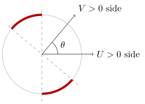
Figure 3: The proof of Lemma 3.3(a). The point \((G_1,G_2)\) has a uniformly random direction. \(U>0\) when this direction lies in the half-circle to the right of the vertical dashed line, and \(V>0\) when it lies in the same half-circle rotated by \(\theta=\arccos\rho\). The signs differ exactly on the two thick arcs, each of length \(\theta\).
Proof. If \(\rho=1\), then \(\sum_w(a_w-b_w)^2=2-2\rho=0\), so \(U=V\), \(\mathbb{P}(UV\le0)=\mathbb{P}(U=0)=0\) by (P2), and the event of (b) is empty. Let \(\rho<1\) and \(\theta=\arccos\rho\in(0,\pi)\).
(a) We write \(V\) in terms of \(U\) and a second, independent normal variable. Put \(a'_w=(b_w-\rho a_w)/\sin\theta\). Then \(\sum_wa_wa'_w=0\) and \(\sum_wa'^2_w=(1-2\rho^2+\rho^2)/\sin^2\theta=1\), so \(G_1=U\) and \(G_2=\sum_wa'_wZ_w\) are standard normal (P2) and independent (P3), and \(V=\cos\theta\,G_1+\sin\theta\,G_2\). Write the point \((G_1,G_2)\) as \(r(\cos\phi,\sin\phi)\) with \(r\ge0\). By (P4) the angle \(\phi\) is uniform on the circle, and \(U=r\cos\phi\) and \(V=r\cos(\phi-\theta)\). Ignoring the outcomes where \(U=0\) or \(V=0\), which have probability \(0\) by (P2), \(U>0\) exactly when \(\phi\) lies in the open half-circle centred at angle \(0\), and \(V>0\) exactly when \(\phi\) lies in the half-circle centred at angle \(\theta\), which is the first one rotated by \(\theta\). So \(UV<0\) exactly when \(\phi\) lies in one of the two half-circles but not the other. As Figure 3 shows,1 this set consists of two arcs of length \(\theta\), so \(\mathbb{P}(UV\le0)=2\theta/(2\pi)=\arccos(\rho)/\pi\).
(b) We compare the threshold \(t\) with the threshold \(0\), in four steps.
Step 1. Let \(S=\frac{U+V}2\) and \(D=\frac{U-V}2\). These are sums of the \(Z_w\) with coefficients \(\frac{a_w+b_w}2\) and \(\frac{a_w-b_w}2\), and \(\sum_w\frac{(a_w+b_w)(a_w-b_w)}4=\frac14\bigl(\sum_wa_w^2-\sum_wb_w^2\bigr)=0\). So \(S\) and \(D\) are independent by (P3). Also \(\mathop{\mathrm{Var}}S=\frac{1+\rho}2>0\), so \(S\) has a density \(f\) that is symmetric and decreasing in \(|s|\) (P2).
Step 2. The event of (b) implies \((U-t)(V-t)\le0\), and \((U-t)(V-t)=(S-t)^2-D^2\). So its probability is at most \(\mathbb{P}(|S-t|\le|D|)\).
Step 3. An interval of given length has the largest mass under \(f\) when it is centred at \(0\): for all \(c\in\mathbb{R}\) and \(w\ge0\), \(\int_{c-w}^{c+w}f\le\int_{-w}^wf\). Indeed, for \(c\ge0\) the difference of the two sides is \(\int_0^c\bigl(f(u+w)-f(u-w)\bigr)\,du\le0\), as \(|u+w|\ge|u-w|\) for \(u\ge0\), and the case \(c<0\) follows by symmetry.
Step 4. Fix a value of \(D\). Since \(S\) is independent of \(D\), the probability that \(|S-t|\le|D|\) is then the mass of the interval \([t-|D|,t+|D|]\) under \(f\), which by Step 3 is at most the mass of \([-|D|,|D|]\). Averaging over the values of \(D\) gives \(\mathbb{P}(|S-t|\le|D|)\le\mathbb{P}(|S|\le|D|)=\mathbb{P}(UV\le0)\), since \(UV=S^2-D^2\). Now (a) finishes the proof. ∎
Fix an integer \(R\ge1\). For vertices \(v,w\) define the coefficient \(c_v(w)\) and, for vertices \(u,v\), the overlap \(\sigma(u,v)\) by \[c_v(w)= \begin{cases}2^{-\mathop{\mathrm{dist}}(v,w)/2}&\text{if }w\in B_R(v),\\0&\text{otherwise,} \end{cases} \qquad \sigma(u,v)=\sum_{w\in V(G)}c_u(w)\,c_v(w).\] We call \(c_v(w)^2=2^{-\mathop{\mathrm{dist}}(v,w)}\) the weight of \(w\) seen from \(v\). So \(\sigma(u,v)\) is a weighted count of the vertices of \(B_R(u)\cap B_R(v)\), and \(\sigma(v,v)=\sum_{k=0}^R2^{-k}\,|\{w:\mathop{\mathrm{dist}}(v,w)=k\}|\) is the total weight of the ball around \(v\). In Section 3.4 the label of \(v\) will be \(Y_v=\sigma(v,v)^{-1/2}\sum_wc_v(w)Z_w\). By (P2), the correlation of the labels of \(u\) and \(v\) will then be \(\sigma(u,v)/\sqrt{\sigma(u,u)\sigma(v,v)}\). The decay \(2^{-k/2}\) of the coefficients balances the spheres: in the \(3\)-regular tree the sphere of radius \(k\ge1\) around \(v\) has \(3\cdot2^{k-1}\) vertices, so every sphere carries the same total weight \(\frac32\), and passing from \(v\) to a neighbor loses only part of the outermost of the \(R\) spheres. The third lemma shows that this holds in every graph of maximum degree \(3\), with no assumption on girth, regularity or connectivity. The same coefficients \((d-1)^{-k/2}\) on spheres are the test functions in Nilli’s proof of the Alon–Boppana bound on the second eigenvalue of \(d\)-regular graphs (Nilli 1991), and the constant \(\frac{2\sqrt2}3\) below is the norm \(2\sqrt2\) of the adjacency operator of the \(3\)-regular tree divided by the degree.
Lemma 3.4 (short edges). Let \(G\) be a graph with \(\Delta(G)\le3\) and let \(R\ge1\) be an integer. Then every edge \(uv\) of \(G\) satisfies \(\sigma(u,v)\ge r_R\sqrt{\sigma(u,u)\,\sigma(v,v)}\), where \(r_R=\frac{2\sqrt2}3\bigl(1-\frac1R\bigr)\).
Proof. The proof has two steps: every shared vertex contributes to \(\sigma(u,v)\) nearly its full weight from both ends, and the vertices that are not shared carry at most a \(\frac1R\) fraction of the weight. Write \(a_w=c_u(w)\), \(b_w=c_v(w)\) and \(I=B_R(u)\cap B_R(v)\). The coefficients are nonnegative and vanish outside the balls, so \(\sigma(u,v)=\sum_{w\in I}a_wb_w\). For \(w\in I\) the distances from \(u\) and from \(v\) to \(w\) differ by at most \(1\), so \(\lambda=a_w/b_w\in[2^{-1/2},2^{1/2}]\); hence \(\lambda+\frac1\lambda\le\frac3{\sqrt2}\), that is, \(a_w^2+b_w^2\le\frac3{\sqrt2}a_wb_w\). Summing over \(I\), with \(A=\sum_{w\in I}a_w^2\) and \(B=\sum_{w\in I}b_w^2\) the weights of the shared vertices seen from \(u\) and from \(v\), and using \(A+B\ge2\sqrt{AB}\), \[\sigma(u,v)\ \ge\ \frac{\sqrt2}{3}(A+B)\ \ge\ \frac{2\sqrt2}{3}\sqrt{AB}.\] It remains to show that the shared vertices carry almost all the weight, that is, \(A\ge(1-\frac1R)\sigma(u,u)\) and \(B\ge(1-\frac1R)\sigma(v,v)\). Let \(s_j\) be the number of vertices at distance \(j\) from \(u\). For \(j\ge1\), a vertex at distance \(j\) has a neighbor at distance \(j-1\) and hence at most two neighbors at distance \(j+1\), so \(s_{j+1}\le2s_j\), and the sphere weights \(s_j2^{-j}\) are nonincreasing in \(j\ge1\). A vertex \(w\in B_R(u)\setminus I\) has \(\mathop{\mathrm{dist}}(v,w)>R\) and hence \(\mathop{\mathrm{dist}}(u,w)\ge\mathop{\mathrm{dist}}(v,w)-1\ge R\), so it lies on the sphere of radius \(R\). Since \(\sigma(u,u)=1+\sum_{j=1}^Rs_j2^{-j}\), \[\sigma(u,u)-A\ \le\ s_R2^{-R}\ \le\ \frac1R\sum_{j=1}^Rs_j2^{-j}\ \le\ \frac1R\,\sigma(u,u),\] and likewise \(\sigma(v,v)-B\le\frac1R\sigma(v,v)\). Hence \(\sigma(u,v)\ge r_R\sqrt{\sigma(u,u)\,\sigma(v,v)}\). ∎
The last lemma is the variance bound for sums of locally dependent terms.
Lemma 3.5 (local sums). Let \(G\) be a graph with \(\Delta(G)\le3\), let \((Z_w)_{w\in V(G)}\) be independent random variables, let \(\ell\ge0\) be an integer and \(\alpha>0\), and let \(Q=\sum_{v\in V(G)}I_v\), where each \(I_v\) takes values in \([0,\alpha]\) and is a function of \((Z_w)_{w\in B_\ell(v)}\). Then \(\mathop{\mathrm{Var}}Q\le\frac34\alpha^2\,4^{\ell}\,n\).
Proof. We use (P1) throughout. We have \(\mathop{\mathrm{Var}}Q=\sum_{u,v}\mathop{\mathrm{Cov}}(I_u,I_v)\). If \(B_\ell(u)\cap B_\ell(v)=\emptyset\), then \(I_u\) and \(I_v\) are functions of disjoint sets of independent variables, hence independent, and \(\mathop{\mathrm{Cov}}(I_u,I_v)=0\). Otherwise \(\mathop{\mathrm{dist}}(u,v)\le2\ell\) and \(|\mathop{\mathrm{Cov}}(I_u,I_v)|\le\sqrt{\mathop{\mathrm{Var}}I_u\mathop{\mathrm{Var}}I_v}\le\frac{\alpha^2}4\), because a variable \(X\) with values in \([0,\alpha]\) has \(\mathop{\mathrm{Var}}X\le\mathbb{E}(X-\frac\alpha2)^2\le\frac{\alpha^2}4\). Since \(\Delta(G)\le3\), every ball satisfies \(|B_{2\ell}(u)|\le1+\sum_{j=1}^{2\ell}3\cdot2^{j-1}<3\cdot4^{\ell}\), so at most \(3\cdot4^\ell n\) pairs \((u,v)\) contribute. ∎
3.4 Proof of Theorem 3.1
Let \(G\) be a graph with \(\Delta(G)\le3\), so that \(m\le\frac32n\), and fix integers \(R,K\ge1\). Let \(Z=(Z_w)_{w\in V(G)}\) have independent standard normal coordinates and give every vertex \(v\) the label \[Y_v=\frac1{\sqrt{\sigma(v,v)}}\sum_{w\in V(G)}c_v(w)\,Z_w ,\] a weighted sum of the independent normal numbers in the ball \(B_R(v)\). By (P2), \(Y_v\) is standard normal and \(\mathop{\mathrm{Corr}}(Y_u,Y_v)=\sigma(u,v)/\sqrt{\sigma(u,u)\sigma(v,v)}\), and every pair \((Y_u,Y_v)\) has the form of Lemma 3.3 with \(a_w=c_u(w)/\sqrt{\sigma(u,u)}\) and \(b_w=c_v(w)/\sqrt{\sigma(v,v)}\). For \(t\in\mathbb{R}\) let \(S_t=\{v:Y_v\le t\}\) and \(e_t=e(S_t)\); an edge \(uv\) crosses \(t\) if exactly one of its ends lies in \(S_t\), that is, if \(\min(Y_u,Y_v)\le t<\max(Y_u,Y_v)\).
Distinct labels. We need the labels to be distinct, so that sorting by label gives an order in which every prefix is a set \(S_t\). Let \(u\ne v\). Among the coefficients of the \(Z_w\) in \(Y_u\) the largest is the one of \(Z_u\), uniquely, and in \(Y_v\) it is the one of \(Z_v\); so the two coefficient sequences differ. Hence \(Y_u-Y_v\) is a normal variable with positive variance, so \(\mathbb{P}(Y_u=Y_v)=0\) by (P2). So all labels are distinct with probability \(1\).
One threshold. By Lemma 3.4 and Lemma 3.3(b), and since \(\arccos\) is decreasing, every edge crosses every threshold with probability at most \(\arccos(r_R)/\pi\). Summing over the \(m\le\frac32n\) edges (linearity of expectation, (P1)) gives \[\begin{equation*} \tag{3.1} \mathbb{E}e_t\le\beta_Rn\quad\text{for every }t\in\mathbb{R},\qquad \beta_R=\frac{3}{2\pi}\arccos r_R . \end{equation*}\] Since \(|\frac{d}{dx}\arccos x|=(1-x^2)^{-1/2}\le3\) for \(0\le x\le\frac{2\sqrt2}3\) and \(\frac{2\sqrt2}3-r_R=\frac{2\sqrt2}{3R}\), the mean value theorem gives \(\beta_R\le c_*+\frac3{2\pi}\cdot3\cdot\frac{2\sqrt2}{3R}=c_*+\frac{3\sqrt2}{\pi R}\).
From one threshold to all thresholds. The bound (3.1) holds for each threshold separately, on average over the random numbers. We need one outcome in which all thresholds are good at the same time, and there are infinitely many thresholds. So we first reduce them to finitely many counts on a grid, then show that each count is close to its mean with high probability, and finally use the union bound (P6).
A grid of thresholds. Labels outside \([-3,3]\) are rare (Section 3.2), so the grid only needs to cover \([-3,3]\). Let \(\tau_j=-3+j/K\) for \(0\le j\le6K\), and for an outcome of the labels let \(N_j=|\{v:\tau_j<Y_v\le\tau_{j+1}\}|\), \(C_-=|\{v:Y_v\le-3\}|\) and \(C_+=|\{v:Y_v>3\}|\). Let \(\tau_j\le\tau<\tau_{j+1}\). An edge \(ab\) with \(Y_a\le\tau<Y_b\) either has \(Y_a\le\tau_j\), and then it is counted by \(e_{\tau_j}\), or has \(\tau_j<Y_a\le\tau<\tau_{j+1}\), and then \(a\) is one of the \(N_j\) counted vertices, each the end of at most three edges. Hence \(e_\tau\le e_{\tau_j}+3N_j\). In the same way \(e_\tau\le3C_-\) for \(\tau<-3\), where the lower end of a crossing edge has label at most \(\tau<-3\), and \(e_\tau\le3C_+\) for \(\tau\ge3\), where the upper end has label greater than \(3\).
Concentration. Consider the \(12K+2\) counts \(e_{\tau_j}\) and \(N_j\) for \(0\le j<6K\), \(C_-\) and \(C_+\). Each label \(Y_u\) is a function of \((Z_w)_{w\in B_R(u)}\). So \(e_\tau=\sum_v|\{u\in N(v):Y_v\le\tau<Y_u\}|\), which counts every crossing edge at its lower end, is a sum over \(v\) of \([0,3]\)-valued functions of \((Z_w)_{w\in B_{R+1}(v)}\), and so are \(N_j\), \(C_-\) and \(C_+\). By Lemma 3.5 with \(\alpha=3\) and \(\ell=R+1\), each count has variance at most \(27\cdot4^Rn\), so by Chebyshev’s inequality (P5) it deviates from its mean by at least \(n^{7/8}\) with probability at most \(27\cdot4^Rn^{-3/4}\). If \[\begin{equation*} \tag{3.2} (12K+2)\cdot27\cdot4^R<n^{3/4}, \end{equation*}\] then the probability that some count deviates from its mean by \(n^{7/8}\) or more is less than \(1\). So by (P6) some outcome of the numbers \(Z_w\) has distinct labels and all \(12K+2\) counts within \(n^{7/8}\) of their means; fix such an outcome. Each \(Y_v\) is standard normal, and its density is at most \(\varphi(0)\), so it lies in an interval of length \(\frac1K\) with probability at most \(\varphi(0)/K\). Hence \(\mathbb{E}N_j\le\varphi(0)n/K\), and \(\mathbb{E}C_\pm=\Phi(-3)n\). By (3.1) and the grid, every \(\tau\in[-3,3)\) satisfies \[e_\tau\ \le\ \Bigl(\beta_R+\frac{3\varphi(0)}K\Bigr)n+4n^{7/8},\] and every \(\tau\notin[-3,3)\) satisfies \(e_\tau\le3\Phi(-3)n+3n^{7/8}\), which is smaller, because \(3\Phi(-3)<0.005<c_*\le\beta_R\).
Conclusion. Order \(V(G)\) by increasing label in the fixed outcome. Every prefix of this ordering is a set \(S_t\), so by Lemma 3.2 \[\mathop{\mathrm{pw}}(G)\ \le\ \operatorname{cw}(G)\ \le\ \max_te_t\ \le\ \Bigl(\beta_R+\frac{3\varphi(0)}K\Bigr)n+4n^{7/8}.\] Take \(K=R=\lfloor\frac14\log_2n\rfloor\). Then \(4^R\le\sqrt n\) and \(12K+2\le3\log_2n+2\), so (3.2) follows from \(27(3\log_2n+2)<n^{1/4}\), which holds for all \(n\ge2^{48}\) (at \(n=2^{48}\) it reads \(3942<4096\)). For \(2^{46}\le n<2^{48}\) we have \(K=R=11\), and (3.2) reads \(134\cdot27\cdot4^{11}<n^{3/4}\), which holds since \(134\cdot27<2^{12}\) and \(2^{12}\cdot2^{22}=2^{34}<2^{34.5}\le n^{3/4}\). So (3.2) holds for all \(n\ge2^{46}\). For these \(n\), since \(\frac{3\sqrt2}\pi+3\varphi(0)<2.55\), \[\mathop{\mathrm{pw}}(G)\ \le\ \operatorname{cw}(G)\ \le\ c_*n+\frac{2.55}Rn+4n^{7/8}\ =\ c_*n+o(n).\] For \(n<2^{46}\) the bound \(\operatorname{cw}(G)\le m\le\frac32n\) is absorbed by the remainder. ◻
3.5 Larger maximum degree
The cut sweep extends to every maximum degree. For an integer \(p\ge3\) put \[r_{pp}=\frac{2\sqrt{p-1}}{p}\qquad\text{and}\qquad \gamma_p=\frac{\arccos r_{pp}}{\pi},\] so that \(r_{33}=\frac{2\sqrt2}3\), \(r_{44}=\frac{\sqrt3}2\), \(r_{55}=\frac45\), and \(\gamma_3=\frac23c_*\approx0.10817\), \(\gamma_4=\frac16\) and \(\gamma_5<0.20484\).
Theorem 3.6 (cut sweep, maximum degree \(p\)). For every integer \(p\ge3\) there is a function \(\eta_p(n)=o(n)\) such that every graph \(G\) with \(\Delta(G)\le p\) satisfies \[\mathop{\mathrm{pw}}(G)\ \le\ \operatorname{cw}(G)\ \le\ \gamma_p\,m+\eta_p(n).\] In particular, the bisection width and the cutwidth of every graph \(G\) with \(\Delta(G)\le4\) are at most \(\frac m6+o(n)\le\frac n3+o(n)\), and those of every graph \(G\) with \(\Delta(G)\le5\) are at most \(\gamma_5m+o(n)\le\frac52\gamma_5n+o(n)<0.5121n+o(n)\).
Proof. We follow Section 3.4 and list the changes. Here and below, \(O_p(\cdot)\) hides constants that depend on \(p\). Let \(c_v(w)=(p-1)^{-\mathop{\mathrm{dist}}(v,w)/2}\) for \(w\in B_R(v)\), and \(c_v(w)=0\) otherwise, and define \(Y_v\) from \(c_v\) as in Section 3.4. Then every edge \(uv\) satisfies \(\mathop{\mathrm{Corr}}(Y_u,Y_v)\ge r_{pp}(1-\frac1R)\): the proof of Lemma 3.4 goes through with \(2\) replaced by \(p-1\), the ratio \(\lambda\in[(p-1)^{-1/2},(p-1)^{1/2}]\), \(\lambda+\frac1\lambda\le\frac2{r_{pp}}\), and \(s_{j+1}\le(p-1)s_j\). (These are the padded labels of Definition 5.2(a), and the bound is Lemma 5.4.) The labels are distinct with probability \(1\), as before.
One threshold. By Lemma 3.3(b), every edge crosses every threshold with probability at most \(\arccos(r_{pp}(1-\frac1R))/\pi\), so \(\mathbb{E}e_t\le\frac m\pi\arccos(r_{pp}(1-\frac1R))\) for every \(t\). On \([0,r_{pp}]\) the derivative of \(\arccos\) has absolute value at most \((1-r_{pp}^2)^{-1/2}=\frac p{p-2}\), and \(m\le\frac p2n\), so \[\mathbb{E}e_t\ \le\ \gamma_p\,m+\frac{p^2r_{pp}}{2\pi(p-2)}\cdot\frac nR\qquad\text{for every }t\in\mathbb{R}.\]
Grid and tails. With the grid of Section 3.4, an edge crossing \(\tau\in[\tau_j,\tau_{j+1})\) either crosses \(\tau_j\) or has its lower end among the \(N_j\) counted vertices, each the end of at most \(p\) edges, so \(e_\tau\le e_{\tau_j}+pN_j\). For the tails we weight by degree, so that the bound stays proportional to \(m\): let \(C'_-=\sum_{v:\,Y_v\le-3}d(v)\) and \(C'_+=\sum_{v:\,Y_v>3}d(v)\). Then \(e_\tau\le C'_-\) for \(\tau<-3\) and \(e_\tau\le C'_+\) for \(\tau\ge3\), and \(\mathbb{E}C'_\pm=2m\Phi(-3)\).
Concentration. The counts \(e_{\tau_j}\), \(N_j\) and \(C'_\pm\) are sums over \(v\) of \([0,p]\)-valued functions of \((Z_w)_{w\in B_{R+1}(v)}\). The proof of Lemma 3.5 applies with \(|B_{2\ell}(u)|\le1+\sum_{j=1}^{2\ell}p(p-1)^{j-1} \le\frac p{p-2}(p-1)^{2\ell}\), so each count has variance at most \(\frac{p^3}{4(p-2)}(p-1)^{2R+2}n\). Take \(K=R=\lfloor\frac18\log_{p-1}n\rfloor\), so that \((p-1)^{2R}\le n^{1/4}\). By Chebyshev’s inequality and a union bound over the \(12K+2\) counts, with probability at least \(1-O_p(n^{-1/2}\log n)\) all of them lie within \(n^{7/8}\) of their means, and then every \(\tau\in[-3,3)\) satisfies \[e_\tau\ \le\ \gamma_pm+\Bigl(\frac{p^2r_{pp}}{2\pi(p-2)}+p\,\varphi(0)\Bigr)\frac nR +(p+1)n^{7/8},\] while every \(\tau\notin[-3,3)\) satisfies \(e_\tau\le2\Phi(-3)m+n^{7/8}\), which is smaller because \(2\Phi(-3)<0.003<\gamma_3\le\gamma_p\). As in Section 3.4, ordering the vertices by their labels gives \(\mathop{\mathrm{pw}}(G)\le\operatorname{cw}(G)\le\max_te_t\), and the error terms are \(O_p(n/R)+(p+1)n^{7/8}=o(n)\), since \(R\to\infty\); for the finitely many \(n\) below the threshold where the probability is positive, \(\operatorname{cw}(G)\le m\le\frac p2n\) is absorbed into \(\eta_p\).
For the bisection width, the first \(\lfloor n/2\rfloor\) vertices of the ordering form a set \(X\) with \(e(X)\le\operatorname{cw}(G)\). For \(p=4\) we have \(r_{44}=\cos\frac\pi6\), so \(\gamma_4=\frac16\), and \(m\le2n\); for \(p=5\), \(m\le\frac52n\) and \(\frac52\gamma_5<0.5121\). ∎
The proof is a randomized polynomial-time algorithm. The labels need the balls of radius \(R=O(\log n)\), which have polynomial size, and the cut values of an ordering can be computed in polynomial time and compared with the explicit bound in the display above. So repeating with fresh Gaussians until the bound holds computes, in expected polynomial time, an ordering of cutwidth at most \(\gamma_pm+o(n)\), for every \(p\ge3\). Since the algorithm checks the bound on the ordering it outputs, its answer is correct whatever numbers it samples; sampling the Gaussians to finite precision can affect only the success probability of a round, which we do not analyze. For \(p\in\{4,5\}\), Theorem 10.3 in Section 10.2 derandomizes it with the method of conditional expectations and computes an ordering of cutwidth at most \(\gamma_pm+o(n)\), and a bisection with at most that many edges between its sides, in deterministic time \(n^{2+o(1)}\).
For \(p=3\), Theorem 3.6 gives \(\gamma_3m\le c_*n\), which Theorem 3.1 states, and the stronger Corollary 1.2 gives \(c_{3}n\). For \(p=4\) the pathwidth bound of Theorem 3.6, \(\frac n3\), is weaker than \(F_4n\) (Theorem 7.1), but the bounds on bisection width and cutwidth are new: Monien and Preis (Monien and Preis 2006 Theorem 2) proved that \(4\)-regular graphs have bisection width at most \(\frac{2n}5+o(n)\), and for maximum degree \(4\) the relations between cutwidth and pathwidth (Makedon and Sudborough 1989 Theorem 3.2; Ellis, Sudborough, and Turner 1994 Theorem 2.1) give only \(\operatorname{cw}(G)\le2\mathop{\mathrm{pw}}(G)+O(1)\le2F_4n+o(n)\).
3.6 Remarks
The argument loses in two places. First, the angle: on cubic graphs of girth greater than \(2R+3\), where every ball \(B_{R+1}(v)\) induces a tree, no choice of coefficients \(c_v(w)\) supported on balls of radius \(R\) and depending only on \(\mathop{\mathrm{dist}}(v,w)\) does better than \(\arcsin\frac13\). There the edge correlations of such labels are those of the \(3\)-regular tree, at most \(\frac{2\sqrt2}3\) because the adjacency operator of that tree has norm \(2\sqrt2\) (Remark 5.1); so at least \(c_*n\) edges cross the median in expectation, and counting crossing edges cannot give a smaller constant with such labels. Second, the count: a vertex of \(N(S_t)\setminus S_t\) is counted once for every neighbor in \(S_t\). Counting each such vertex once needs the joint distribution of a label and all its neighbor labels, in which the correlations between two neighbors are unknown; the star comparison of Section 6 handles them and gives the plain-sweep constant \(F_3\approx0.14016\) (Theorem 7.1(b) with \(n_4=0\)), and switching from inner to outer frontiers at threshold \(0\) gives \(c_{3}\) (Theorem 8.1). Finally, for graphs that converge locally to the \(3\)-regular tree (for example, cubic graphs of large girth), \(c_*\) is the density of the sign cut (threshold \(0\)) of the Gaussian wave (Lyons 2017).
The edge isoperimetric number.
For a \(d\)-regular graph the bisection of Theorem 3.6 gives the edge isoperimetric number \(i(G)=\min\{e(S)/|S|:0<|S|\le\frac n2\}\), where \(e(S)\) is the number of edges with exactly one end in \(S\), at most \(d\gamma_d+o(1)\le\frac d2-\frac2\pi\sqrt{d-1}+o(1)\). Alon’s upper bound has the form \(\frac d2-c\sqrt d\) for \(n>n_0(d)\), with \(c=\frac3{16\sqrt2}<0.133\) (Alon 1997 Theorem 1.1 and (11)); for \(d\ge3\) and \(n\) large enough, our bound gives \(\frac2\pi\sqrt{d-1}>0.51\sqrt d\) in place of \(c\sqrt d\). For cubic graphs, Corollary 1.2 gives \(i(G)\le2c_{3}+o(1)<0.2797\), in place of the bound \(\frac13\) that follows from the theorem of Monien and Preis (Monien and Preis 2006 Theorem 1), and \(4\)-regular graphs have \(i(G)\le\frac23+o(1)\).
References
Footnotes
Part (a) also has a proof by calculus alone. For \(-1<\rho<1\) let \(P(\rho)=\mathbb{P}(U>0,\,V>0)\). By Plackett’s identity (Plackett 1954) for two variables, \(P'(\rho)\) is the joint density of \((U,V)\) at \((0,0)\), which is \(1/(2\pi\sqrt{1-\rho^2})\). Since \(P(0)=\frac14\), integration gives \(P(\rho)=\frac14+\frac{\arcsin\rho}{2\pi}\), and by symmetry \(\mathbb{P}(UV\le0)=1-2P(\rho)=\frac{\arccos\rho}\pi\).↩︎